Optimizers
Level 6 · Chapter 4 · ⏱️ ~75 min read · Prerequisites: A neural network in NumPy, Gradient descent in depth
An optimizer decides how a gradient becomes a step. This chapter implements the optimizers you'll meet in every deep learning codebase, from scratch: SGD, momentum and Nesterov momentum, AdaGrad, RMSProp, Adam with its bias correction, and AdamW with decoupled weight decay. You'll race them on the Rosenbrock function, where you can watch their paths, and on the digits network from the previous chapter, then add learning-rate schedules (step decay, cosine annealing, and warmup), and check your implementations against PyTorch's.
Why it matters
Alex's team was reproducing a published image classifier. The paper said "trained with learning rate 0.1," and the team, who used Adam for everything, set Adam's learning rate to 0.1. The loss went to nan in the first hundred steps. They lowered it to 0.01; the loss went down for a while and then the network collapsed to predicting one class. At 0.001 it trained, but ended three points below the paper.
The paper had used SGD with momentum, not Adam, and a cosine learning-rate schedule. A learning rate of 0.1 is normal for SGD with momentum and wildly too large for Adam, because the two optimizers interpret the number completely differently: SGD multiplies it by the gradient, while Adam uses it as an approximate step size per parameter. Once the team matched the optimizer and its schedule, they reproduced the result in one run.
The optimizer, its learning rate, and the schedule are a single unit. To set them sensibly, you need to know what each optimizer does with a gradient.
Concepts
Why plain gradient descent struggles
The loss surface of a neural network is non-convex, high-dimensional, and seen only through noisy mini-batch gradients. Three features of it make plain gradient descent slow:
- Ravines. In some directions the loss curves sharply; in others it's nearly flat. You saw this in Gradient descent in depth: with condition number \(\kappa\) (the ratio of the largest to the smallest curvature), gradient descent needs on the order of \(\kappa\) steps, because a learning rate small enough to be stable in the steep direction crawls in the flat one.
- Different scales per parameter. Gradients for some weights (say, those attached to rare features or to early layers) are consistently much smaller than for others. A single learning rate is too small for some parameters and too big for others.
- Noise. Mini-batch gradients point in the right direction only on average. Near a minimum, the noise dominates, and a constant learning rate makes the parameters jitter around it instead of settling.
Each optimizer below fixes one or more of these. Write \(\mathbf{g}_t = \nabla_\theta\mathcal{L}(\theta_{t-1})\) for the (mini-batch) gradient at step \(t\), \(\eta\) for the learning rate, and treat all operations on vectors, including squares, square roots, and division, as element-wise.
SGD, revisited
Stochastic gradient descent is the baseline:
It's simple, needs no extra memory, and with a well-tuned learning rate and schedule it's still competitive for many vision models. Its step is proportional to the gradient: large where the loss is steep, tiny where it's flat. That's exactly wrong in a ravine, where the steep direction is the one to be careful in and the flat direction is the one you need to travel.
Momentum
Momentum keeps a running velocity \(\mathbf{v}\), a decaying sum of past gradients, and steps along it. You previewed it in Gradient descent in depth:
with \(\mathbf{v}_0 = \mathbf{0}\) and momentum coefficient \(\beta\), usually 0.9.
Intuition. A heavy ball rolling down a ravine. Across the ravine, consecutive gradients point in opposite directions, so they cancel in the velocity. Along the ravine, they all point the same way, so they add up. Unrolling the recursion shows what the velocity is:
If the gradient were a constant \(\mathbf{g}\), the velocity would approach \(\mathbf{g}\sum_k\beta^k = \frac{\mathbf{g}}{1 - \beta}\). So in a consistent direction, momentum multiplies the effective learning rate by \(\frac{1}{1 - \beta}\): 10 times for \(\beta = 0.9\). That's worth remembering when you switch between SGD with and without momentum: SGD with momentum at \(\eta = 0.01\) behaves roughly like plain SGD at \(\eta = 0.1\) along consistent directions, but without the oscillation across the ravine.
(Some texts write \(\mathbf{v}_t = \beta\mathbf{v}_{t-1} + (1 - \beta)\mathbf{g}_t\), an exponential moving average. That's the same method with the learning rate rescaled by \(1 - \beta\). PyTorch uses the form above.)
Nesterov momentum
Momentum has a flaw: the ball commits to its velocity before looking where it's going. If the velocity carries it past the bottom of a valley, it only finds out on the next step. Nesterov accelerated gradient (NAG) evaluates the gradient at the point momentum is about to carry you to, the lookahead point:
If the momentum step would overshoot, the gradient at the lookahead point already points back, and the correction happens one step earlier. For convex problems, Yurii Nesterov proved in 1983 that this improves the worst-case convergence rate of gradient methods; for neural networks, it's a modest, fairly reliable improvement over plain momentum.
Computing a gradient at a different point from the current parameters is awkward in code. A change of variables (track the lookahead point as "the parameters") gives the equivalent form that PyTorch implements, which only needs the gradient at the current parameters:
Compare it with ordinary momentum: the step uses \(\mathbf{g}_t + \beta\mathbf{v}_t\) instead of \(\mathbf{v}_t = \mathbf{g}_t + \beta\mathbf{v}_{t-1}\). It's as if the velocity were applied one step ahead.
AdaGrad: a learning rate per parameter
Momentum fixes the direction; it doesn't fix scale differences between parameters. AdaGrad (Duchi, Hazan, and Singer, 2011) gives each parameter its own learning rate, shrinking it for parameters that have seen large gradients:
\(\mathbf{G}_t\) accumulates the squared gradients of each parameter over all of training, and the small constant \(\epsilon\) (like \(10^{-8}\) or \(10^{-10}\)) prevents division by zero.
Intuition. Dividing by the root of the accumulated squared gradient normalizes the step: a parameter with consistently large gradients gets a small effective learning rate, and a parameter with rare or small gradients gets a large one. That's ideal for sparse features, like rare words in a text model, which get few updates and need each to count. It also makes the method nearly invariant to the scale of the gradient: multiply the loss by 100, and both \(\mathbf{g}\) and \(\sqrt{\mathbf{G}}\) scale by 100, leaving the step unchanged.
The flaw. \(\mathbf{G}_t\) only grows, so the effective learning rate decays forever. With a constant gradient \(g\), \(\sqrt{G_t} = |g|\sqrt{t}\), so the step size falls like \(\eta/\sqrt{t}\). That's sometimes what convex optimization theory wants, but in deep learning the network often stops learning long before it reaches a good solution.
RMSProp
RMSProp (proposed by Geoffrey Hinton in a 2012 lecture, never formally published) fixes AdaGrad's decay by replacing the sum with an exponential moving average, so old gradients are forgotten:
with decay rate \(\rho\) around 0.9 to 0.99. Now \(\sqrt{\mathbf{s}_t}\) is a running estimate of the root mean square of each parameter's recent gradients, hence the name. The effective learning rate adapts up and down as gradient magnitudes change. Because each step divides the gradient by its typical size, a parameter's step is roughly \(\eta\) in magnitude whenever its gradient is consistent, whatever the gradient's raw scale.
Adam
Adam (Kingma and Ba, 2015), short for "adaptive moment estimation," combines both ideas: a momentum-like moving average of the gradient (the first moment) and an RMSProp-like moving average of its square (the second moment):
The defaults, which work surprisingly often, are \(\eta = 10^{-3}\), \(\beta_1 = 0.9\), \(\beta_2 = 0.999\), and \(\epsilon = 10^{-8}\). (\(\beta_1^t\) means \(\beta_1\) raised to the power \(t\), the step count.)
Bias correction. Both moving averages start at zero, which biases them toward zero early in training. Take the expectation of the unrolled first moment, assuming the gradients have a stationary mean \(\mathbb{E}[\mathbf{g}]\):
using the geometric sum \(\sum_{k=0}^{t-1}\beta^k = \frac{1 - \beta^t}{1 - \beta}\). So \(\mathbf{m}_t\) underestimates the mean gradient by the factor \(1 - \beta_1^t\), and dividing by that factor removes the bias. At \(t = 1\) with \(\beta_1 = 0.9\), \(\mathbf{m}_1 = 0.1\,\mathbf{g}_1\), and the correction multiplies by 10. The same argument applies to \(\mathbf{v}_t\) with \(\beta_2\). Because \(\beta_2 = 0.999\) is so close to 1, \(\mathbf{v}_t\)'s bias lasts for thousands of steps, and correcting it matters more. Without the correction, Adam's first steps are distorted: \(\mathbf{m}_1 / \sqrt{\mathbf{v}_1} = 0.1\,g / \sqrt{0.001\,g^2} \approx 3.16\,\operatorname{sign}(g)\), more than three times the intended step size. You'll check this in the code.
What the update does. The ratio \(\hat{\mathbf{m}}_t / \sqrt{\hat{\mathbf{v}}_t}\) is like a signal-to-noise ratio for each parameter. If a parameter's gradient is consistent, \(|\hat{m}| \approx \sqrt{\hat{v}}\), and the step is about \(\eta\). If its gradient is mostly noise, the mean is small relative to the root mean square, and the step shrinks. So \(\eta\) in Adam is roughly a maximum step size per parameter, independent of the loss's scale. In SGD, \(\eta\) multiplies the gradient. That's why the same number means such different things for the two, as Alex's team discovered.
Adam is the default for transformers and many other architectures because it's robust to poorly scaled gradients and needs less learning-rate tuning. Well-tuned SGD with momentum sometimes generalizes slightly better on image classification. Neither is universally better.
Weight decay and AdamW
Weight decay shrinks every weight toward zero a little at each step:
For plain SGD, this is identical to adding an L2 penalty \(\frac{\lambda}{2}\lVert\theta\rVert^2\) to the loss, as in Regularization: the penalty's gradient \(\lambda\theta\) gets multiplied by \(\eta\) and subtracted. So people used the two terms interchangeably.
For adaptive optimizers they're not the same. If you add \(\lambda\theta\) to the gradient before Adam's update, the penalty's gradient gets divided by \(\sqrt{\hat{\mathbf{v}}_t}\) along with everything else. Parameters with large gradient history get their regularization shrunk; parameters with small gradients get it amplified. The regularization strength ends up depending on gradient statistics in ways nobody intended. Ilya Loshchilov and Frank Hutter (2019) showed this hurts generalization and proposed AdamW, which decouples the decay from the adaptive step:
The moments \(\hat{\mathbf{m}}_t, \hat{\mathbf{v}}_t\) are computed from the loss gradient alone. Every weight shrinks by the same fraction \(\eta\lambda\) per step. AdamW, with \(\lambda\) around 0.01 to 0.1, is the standard optimizer for training transformers. In practice, weight decay is usually not applied to biases or normalization parameters, only to weight matrices.
Learning-rate schedules
No single learning rate is right for all of training. Early on, large steps make fast progress. Later, the gradient noise dominates, and large steps keep the parameters bouncing around the minimum. A learning-rate schedule \(\eta_t\) changes the learning rate over the course of training. With \(T\) total steps and peak learning rate \(\eta_{\max}\):
- Step decay multiplies the learning rate by a factor (often 0.1) at fixed milestones, such as 50% and 75% of training: \(\eta_t = \eta_{\max}\cdot\gamma^{\lfloor t / s\rfloor}\) for decay factor \(\gamma\) every \(s\) steps. It was the standard for image classifiers for years; the loss drops visibly at each milestone.
- Exponential decay shrinks it smoothly: \(\eta_t = \eta_{\max}\,\gamma^{t}\) with \(\gamma\) slightly below 1.
- Cosine annealing (Loshchilov and Hutter, 2017) follows half a cosine from \(\eta_{\max}\) down to \(\eta_{\min}\) (often 0):
It stays near the peak for a while, decays fastest in the middle, and lands gently. It has only one shape parameter to choose (\(T\)), and it's a strong default.
- Linear warmup starts the learning rate near zero and ramps it linearly to \(\eta_{\max}\) over the first \(T_w\) steps (often 1% to 10% of training), then hands over to another schedule, usually cosine: \(\eta_t = \eta_{\max}\,t / T_w\) for \(t \leq T_w\).
Why warmup? At initialization, the network is far from any sensible solution, and early gradients can be large and erratic. With Adam, there's a second reason: in the first steps, \(\hat{\mathbf{v}}_t\) is estimated from only a handful of gradients, and as you saw, Adam's step is about \(\eta\) per parameter regardless of the gradient's size. So at step 1, every parameter moves by about \(\eta\) in the direction of a single noisy mini-batch gradient. A full-size learning rate can do lasting damage in those steps, such as killing ReLUs or blowing up a normalization layer's statistics, before the moment estimates become reliable. Warmup keeps the early steps small. It's essential for transformers and for very large batch sizes, and often unnecessary for small networks.
Comparing optimizers fairly
Optimizer comparisons are easy to get wrong. A fair comparison:
- Tunes the learning rate separately for each optimizer. Comparing SGD and Adam at the same learning rate compares nothing, as the opening story showed. Sweep a log-spaced grid (for example, factors of 3) for each and compare the best of each.
- Uses the same budget: the same number of epochs or gradient evaluations, and the same schedule shape.
- Uses several seeds when differences are small, because one run's noise can exceed the difference between optimizers.
- Measures what you care about. Training loss shows how fast an optimizer optimizes; validation performance shows how well the result generalizes. They can rank optimizers differently.
In practice
The optimizers, from scratch
All the optimizers share an interface: construct them with a list of parameter arrays, and call step(grads) with a matching list of gradient arrays. Each optimizer keeps its state (velocities, moment estimates) per parameter and updates the arrays in place, so it works with any code that exposes its parameters, including the layer library from the previous chapter. The lr attribute can be changed between steps by a schedule.
import numpy as np
import matplotlib.pyplot as plt

class Optimizer:
    def __init__(self, params, lr):
        self.params, self.lr, self.t = list(params), lr, 0

    def step(self, grads):
        self.t += 1
        for i, (p, g) in enumerate(zip(self.params, grads)):
            self.update(i, p, g)

    def update(self, i, p, g):
        raise NotImplementedError


class SGD(Optimizer):
    def update(self, i, p, g):
        p -= self.lr * g


class Momentum(Optimizer):
    def __init__(self, params, lr, beta=0.9, nesterov=False):
        super().__init__(params, lr)
        self.beta, self.nesterov = beta, nesterov
        self.v = [np.zeros_like(p) for p in self.params]

    def update(self, i, p, g):
        v = self.v[i]
        v *= self.beta
        v += g                                                  # v_t = beta v_{t-1} + g_t
        p -= self.lr * (g + self.beta * v if self.nesterov else v)


class AdaGrad(Optimizer):
    def __init__(self, params, lr, eps=1e-10):
        super().__init__(params, lr)
        self.eps = eps
        self.G = [np.zeros_like(p) for p in self.params]

    def update(self, i, p, g):
        self.G[i] += g * g                                      # sum of squared gradients
        p -= self.lr * g / (np.sqrt(self.G[i]) + self.eps)


class RMSProp(Optimizer):
    def __init__(self, params, lr, rho=0.9, eps=1e-8):
        super().__init__(params, lr)
        self.rho, self.eps = rho, eps
        self.s = [np.zeros_like(p) for p in self.params]

    def update(self, i, p, g):
        s = self.s[i]
        s *= self.rho
        s += (1 - self.rho) * g * g                             # moving average of g^2
        p -= self.lr * g / (np.sqrt(s) + self.eps)


class Adam(Optimizer):
    def __init__(self, params, lr=1e-3, betas=(0.9, 0.999), eps=1e-8,
                 weight_decay=0.0, decoupled=False, bias_correction=True):
        super().__init__(params, lr)
        self.b1, self.b2 = betas
        self.eps, self.wd, self.decoupled, self.bias_correction = eps, weight_decay, decoupled, bias_correction
        self.m = [np.zeros_like(p) for p in self.params]
        self.v = [np.zeros_like(p) for p in self.params]

    def update(self, i, p, g):
        if self.wd and not self.decoupled:
            g = g + self.wd * p                                 # L2 penalty: goes through the adaptive scaling
        m, v = self.m[i], self.v[i]
        m *= self.b1
        m += (1 - self.b1) * g
        v *= self.b2
        v += (1 - self.b2) * g * g
        if self.bias_correction:
            m_hat, v_hat = m / (1 - self.b1 ** self.t), v / (1 - self.b2 ** self.t)
        else:
            m_hat, v_hat = m, v
        if self.wd and self.decoupled:
            p -= self.lr * self.wd * p                          # AdamW: decay applied directly
        p -= self.lr * m_hat / (np.sqrt(v_hat) + self.eps)


def AdamW(params, lr=1e-3, weight_decay=0.01, **kw):
    return Adam(params, lr, weight_decay=weight_decay, decoupled=True, **kw)
Racing on the Rosenbrock function
The Rosenbrock function is a classic optimizer benchmark:
Its minimum is \(f = 0\) at \((1, 1)\), at the bottom of a long, curved, banana-shaped valley. Finding the valley is easy; following its curved floor is hard, because the valley's walls are about 100 times steeper than its floor. Near the minimum, the Hessian's eigenvalues are about 1,000 and 0.4, a condition number around 2,500.
Each optimizer starts at \((-1.5, 2)\) and runs 3,000 steps, with a learning rate picked from a small sweep for each. AdamW is left out here: it would just add a pull toward the origin, which makes no sense for a function that isn't a neural network's loss.
def rosenbrock(p):
    x, y = p
    return (1 - x) ** 2 + 100 * (y - x ** 2) ** 2

def rosenbrock_grad(p):
    x, y = p
    return np.array([-2 * (1 - x) - 400 * x * (y - x ** 2), 200 * (y - x ** 2)])

def run(make_opt, steps=3000, start=(-1.5, 2.0)):
    p = np.array(start)
    opt = make_opt([p])
    path = [p.copy()]
    for _ in range(steps):
        opt.step([rosenbrock_grad(p)])
        path.append(p.copy())
    return np.array(path)

contenders = {
    "SGD (lr 1e-3)":                lambda ps: SGD(ps, 1e-3),
    "Momentum (lr 1e-3)":           lambda ps: Momentum(ps, 1e-3),
    "Nesterov (lr 1e-3)":           lambda ps: Momentum(ps, 1e-3, nesterov=True),
    "AdaGrad (lr 0.5)":             lambda ps: AdaGrad(ps, 0.5),
    "RMSProp (lr 3e-3)":            lambda ps: RMSProp(ps, 3e-3),
    "Adam (lr 0.03)":               lambda ps: Adam(ps, 0.03),
}
paths = {name: run(make) for name, make in contenders.items()}

print(f"{'optimizer':<22}{'steps to within 0.01':>22}{'final distance':>16}{'final f':>11}")
for name, path in paths.items():
    dist = np.linalg.norm(path - 1.0, axis=1)
    hit = np.argmax(dist < 0.01) if (dist < 0.01).any() else None
    print(f"{name:<22}{str(hit) if hit is not None else 'never':>22}{dist[-1]:>16.1e}{rosenbrock(path[-1]):>11.1e}")

xs, ys = np.meshgrid(np.linspace(-2, 2, 400), np.linspace(-1, 3, 400))
zs = (1 - xs) ** 2 + 100 * (ys - xs ** 2) ** 2
fig, axes = plt.subplots(2, 3, figsize=(13, 8), sharex=True, sharey=True)
for ax, (name, path) in zip(axes.ravel(), paths.items()):
    ax.contour(xs, ys, zs, levels=np.logspace(-1, 3.5, 14), cmap="Greys", linewidths=0.6)
    ax.plot(path[:, 0], path[:, 1], color="tab:blue", lw=1)
    ax.plot(path[::100, 0], path[::100, 1], "o", color="tab:blue", ms=2.5)   # a dot every 100 steps
    ax.plot(-1.5, 2, "ks", ms=5); ax.plot(1, 1, "r*", ms=12)
    ax.set_title(name, fontsize=10)
plt.tight_layout()
plt.show()
optimizer               steps to within 0.01  final distance    final f
SGD (lr 1e-3)                          never         4.5e-01    4.9e-02
Momentum (lr 1e-3)                      1125         4.1e-06    3.3e-12
Nesterov (lr 1e-3)                      1018         2.7e-06    1.5e-12
AdaGrad (lr 0.5)                       never         3.6e-01    3.0e-02
RMSProp (lr 3e-3)                      never         6.0e-02    2.7e-03
Adam (lr 0.03)                          1592         1.5e-08    4.2e-17
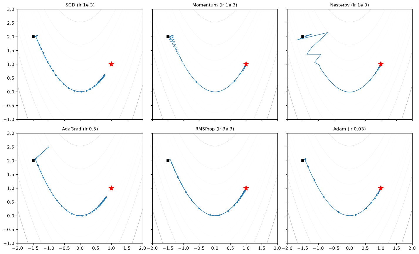
Paths of six optimizers on the Rosenbrock function over 3,000 steps, with a dot every 100 steps. Dense dots mean slow progress.
Each optimizer shows its personality:
- SGD drops into the valley almost immediately (the walls are steep), then crawls along the flat floor. Its learning rate can't be raised, because the steep direction would diverge: near the minimum, stability needs \(\eta < 2/\lambda_{\max} \approx 0.002\).
- Momentum and Nesterov use the same learning rate but build up speed along the floor, reaching the minimum in about 1,000 steps. Both zigzag across the valley at first, where the walls are steepest; Nesterov's early jumps are even wilder (its lookahead gradient is taken where the walls are steeper still), but once on the floor it arrives a little sooner.
- AdaGrad normalizes the steep and flat directions, but its accumulated \(\mathbf{G}_t\) keeps growing and its steps keep shrinking: it's still crawling at step 3,000.
- RMSProp reaches the valley floor fast, but with a constant learning rate its normalized steps never shrink, so it ends up bouncing in a small region short of the minimum. It needs a decaying schedule.
- Adam combines momentum's acceleration with RMSProp's normalization, and its momentum averages away the bouncing; it converges to machine precision.
Don't over-read a 2D benchmark. Rosenbrock is smooth, noiseless, and two-dimensional; a neural network's loss is none of those. The next comparison is closer to real use.
Adam's bias correction in action
With a constant gradient, Adam's step should be exactly \(\eta\) from the very first step. Here are the first steps with and without the bias correction, for a gradient of 0.5 and \(\eta = 0.01\):
for corrected in [True, False]:
    p = np.zeros(1)
    opt = Adam([p], lr=0.01, bias_correction=corrected)
    steps = []
    for t in range(1, 2001):
        before = p.copy()
        opt.step([np.array([0.5])])
        steps.append(float((before - p)[0]))
    label = "with correction   " if corrected else "without correction"
    print(label, "step sizes at t = 1, 2, 3, 10, 100, 2000:",
          [round(steps[t - 1], 4) for t in [1, 2, 3, 10, 100, 2000]])
with correction    step sizes at t = 1, 2, 3, 10, 100, 2000: [0.01, 0.01, 0.01, 0.01, 0.01, 0.01]
without correction step sizes at t = 1, 2, 3, 10, 100, 2000: [0.0316, 0.0425, 0.0495, 0.0653, 0.0324, 0.0108]
Without the correction, the steps start at \(\sqrt{10} \approx 3.16\) times the intended size, grow for a while (the first moment catches up faster than the second), and take thousands of steps to settle back to \(\eta\), exactly as the derivation predicted. With it, every step is \(\eta\).
Optimizers on the digits network
Now a real network: the 64-128-10 ReLU network from the previous chapter, on the same digits split. The layer classes are repeated here so this section runs on its own.
The layer library and data from the previous chapter (expand to copy)
from sklearn.datasets import load_digits
from sklearn.model_selection import train_test_split

digits = load_digits()
X_all, y_all = digits.data / 16.0, digits.target
X_tmp, X_test, y_tmp, y_test = train_test_split(X_all, y_all, test_size=0.2, stratify=y_all, random_state=0)
X_train, X_val, y_train, y_val = train_test_split(X_tmp, y_tmp, test_size=0.25, stratify=y_tmp, random_state=0)

class Linear:
    def __init__(self, d_in, d_out, rng):
        self.params = {"W": rng.normal(0.0, np.sqrt(2.0 / d_in), size=(d_in, d_out)), "b": np.zeros(d_out)}
        self.grads = {}
    def forward(self, X):
        self.X = X
        return X @ self.params["W"] + self.params["b"]
    def backward(self, dout):
        self.grads["W"] = self.X.T @ dout
        self.grads["b"] = dout.sum(axis=0)
        return dout @ self.params["W"].T

class ReLU:
    params, grads = {}, {}
    def forward(self, X):
        self.mask = X > 0
        return X * self.mask
    def backward(self, dout):
        return dout * self.mask

class SoftmaxCrossEntropy:
    def forward(self, logits, y):
        Z = logits - logits.max(axis=1, keepdims=True)
        log_probs = Z - np.log(np.exp(Z).sum(axis=1, keepdims=True))
        self.probs, self.y = np.exp(log_probs), y
        return -np.mean(log_probs[np.arange(len(y)), y])
    def backward(self):
        d = self.probs.copy()
        d[np.arange(len(self.y)), self.y] -= 1.0
        return d / len(self.y)

class Sequential:
    def __init__(self, *layers):
        self.layers = list(layers)
    def forward(self, X):
        for layer in self.layers:
            X = layer.forward(X)
        return X
    def backward(self, dout):
        for layer in reversed(self.layers):
            dout = layer.backward(dout)
    def param_arrays(self):
        return [layer.params[k] for layer in self.layers for k in layer.params]
    def grad_arrays(self):
        return [layer.grads[k] for layer in self.layers for k in layer.params]

def mlp(sizes, seed=0):
    rng = np.random.default_rng(seed)
    layers = []
    for i, (a, b) in enumerate(zip(sizes[:-1], sizes[1:])):
        layers.append(Linear(a, b, rng))
        if i < len(sizes) - 2:
            layers.append(ReLU())
    return Sequential(*layers)

def accuracy(model, X, y):
    return np.mean(model.forward(X).argmax(axis=1) == y)
The training function takes an optimizer factory and an optional schedule, a function of the step number. Note the one design change from the last chapter: the update is now opt.step(model.grad_arrays()).
def fit(make_opt, sizes=(64, 128, 10), epochs=20, batch_size=32, schedule=None, seed=0):
    model = mlp(sizes, seed)
    opt = make_opt(model.param_arrays())
    loss_fn = SoftmaxCrossEntropy()
    rng = np.random.default_rng(seed)
    n = len(X_train)
    total_steps = epochs * int(np.ceil(n / batch_size))
    step, losses = 0, []
    for epoch in range(epochs):
        order, running = rng.permutation(n), 0.0
        for start in range(0, n, batch_size):
            idx = order[start:start + batch_size]
            if schedule is not None:
                opt.lr = schedule(step, total_steps)
            loss = loss_fn.forward(model.forward(X_train[idx]), y_train[idx])
            model.backward(loss_fn.backward())
            opt.step(model.grad_arrays())
            running += loss * len(idx)
            step += 1
        losses.append(running / n)
    return model, losses

lr_grids = {
    "SGD":      (lambda lr: lambda ps: SGD(ps, lr),                      [0.03, 0.1, 0.3, 1, 3]),
    "Momentum": (lambda lr: lambda ps: Momentum(ps, lr),                 [0.003, 0.01, 0.03, 0.1, 0.3]),
    "Nesterov": (lambda lr: lambda ps: Momentum(ps, lr, nesterov=True),  [0.003, 0.01, 0.03, 0.1, 0.3]),
    "AdaGrad":  (lambda lr: lambda ps: AdaGrad(ps, lr),                  [0.01, 0.03, 0.1, 0.3, 1]),
    "RMSProp":  (lambda lr: lambda ps: RMSProp(ps, lr),                  [3e-4, 1e-3, 3e-3, 0.01, 0.03]),
    "Adam":     (lambda lr: lambda ps: Adam(ps, lr),                     [3e-4, 1e-3, 3e-3, 0.01, 0.03]),
    "AdamW":    (lambda lr: lambda ps: AdamW(ps, lr, weight_decay=0.01), [3e-4, 1e-3, 3e-3, 0.01, 0.03]),
}

best = {}
print(f"{'optimizer':<10} " + "  ".join(f"{'lr':>6} {'val':>5}" for _ in range(5)) + "   best lr  train loss")
for name, (factory, lrs) in lr_grids.items():
    results = []
    for lr in lrs:
        model, losses = fit(factory(lr))
        results.append((accuracy(model, X_val, y_val), -losses[-1], lr, losses))
    val_acc, neg_loss, lr, losses = max(results)                  # best validation accuracy, ties -> lower loss
    best[name] = (lr, losses)
    row = "  ".join(f"{r[2]:>6g} {r[0]:.3f}" for r in results)
    print(f"{name:<10} {row}   {lr:>7g}  {-neg_loss:.4f}")
optimizer      lr   val      lr   val      lr   val      lr   val      lr   val   best lr  train loss
SGD          0.03 0.944     0.1 0.958     0.3 0.961       1 0.969       3 0.100         1  0.0066
Momentum    0.003 0.944    0.01 0.961    0.03 0.969     0.1 0.972     0.3 0.967       0.1  0.0058
Nesterov    0.003 0.944    0.01 0.964    0.03 0.964     0.1 0.969     0.3 0.978       0.3  0.0003
AdaGrad      0.01 0.964    0.03 0.967     0.1 0.969     0.3 0.969       1 0.964       0.1  0.0145
RMSProp    0.0003 0.939   0.001 0.964   0.003 0.969    0.01 0.967    0.03 0.964     0.003  0.0151
Adam       0.0003 0.944   0.001 0.967   0.003 0.978    0.01 0.969    0.03 0.967     0.003  0.0249
AdamW      0.0003 0.944   0.001 0.967   0.003 0.975    0.01 0.975    0.03 0.969      0.01  0.0042
Three things stand out.
- Once each learning rate is tuned, the optimizers are close. Every one reaches about 97% to 98% validation accuracy, and the differences between them are about the size of the differences between neighboring learning rates for the same optimizer. On a small, well-conditioned problem like this one, the optimizer matters less than tuning it.
- The best learning rates span more than two orders of magnitude, from 0.003 for Adam and RMSProp to 1 for SGD. And momentum's best (0.1) is 10 times smaller than SGD's (1), matching the \(\frac{1}{1 - \beta} = 10\) effective-learning-rate factor. Notice too that SGD at 3 fails completely (10% is chance): the cliff on the high side of the best learning rate is often steep.
- Training loss and validation accuracy rank differently. Nesterov at 0.3 reaches by far the lowest training loss, while Adam at 0.003 matches its validation accuracy with a training loss nearly 100 times higher. Nesterov's best is also at the edge of its grid, which in a real sweep means you should extend the grid before concluding anything.
With one seed and 360 validation examples, a difference of 0.003 is a single image, so don't rank optimizers on differences that small. (Exercise 6 asks you to measure the seed-to-seed spread.)
Learning-rate schedules
Schedules are functions from the step number to a learning rate. Here are four, scaled to a peak of 0.01:
def constant(peak):
    return lambda t, T: peak

def step_decay(peak, drops=(0.5, 0.75), factor=0.1):
    return lambda t, T: peak * factor ** sum(t >= d * T for d in drops)

def cosine(peak, floor=0.0):
    return lambda t, T: floor + 0.5 * (peak - floor) * (1 + np.cos(np.pi * t / T))

def warmup_cosine(peak, warmup_frac=0.05, floor=0.0):
    def schedule(t, T):
        warm = max(1, int(warmup_frac * T))
        if t < warm:
            return peak * (t + 1) / warm
        return floor + 0.5 * (peak - floor) * (1 + np.cos(np.pi * (t - warm) / (T - warm)))
    return schedule

deep = (64, 256, 256, 256, 10)                       # three hidden layers
schedules = {"constant": constant(0.01), "step decay": step_decay(0.01),
             "cosine": cosine(0.01), "warmup + cosine": warmup_cosine(0.01)}

fig, axes = plt.subplots(1, 2, figsize=(12, 4))
T = 1000
for name, s in schedules.items():
    axes[0].plot([s(t, T) for t in range(T)], label=name)
axes[0].set_xlabel("step"); axes[0].set_ylabel("learning rate"); axes[0].set_title("schedule shapes"); axes[0].legend()

print(f"{'Adam, peak lr 0.01':<18} {'final train loss':>17} {'val acc':>8}")
for name, s in schedules.items():
    model, losses = fit(lambda ps: Adam(ps, 0.01), sizes=deep, schedule=s)
    axes[1].plot(np.arange(1, 21), losses, label=name)
    print(f"{name:<18} {losses[-1]:>17.5f} {accuracy(model, X_val, y_val):>8.3f}")
axes[1].set_yscale("log"); axes[1].set_xlabel("epoch"); axes[1].set_ylabel("training loss")
axes[1].set_title("Adam, 3 hidden layers, peak lr 0.01"); axes[1].legend()
plt.tight_layout()
plt.show()
Adam, peak lr 0.01  final train loss  val acc
constant                     0.04723    0.967
step decay                   0.00062    0.978
cosine                       0.00008    0.975
warmup + cosine              0.00019    0.969
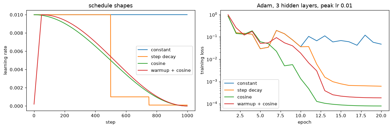
Left: the schedules. Right: training loss with Adam at a peak learning rate of 0.01. A constant learning rate leaves the loss bouncing around a plateau; every decaying schedule lets it settle much lower, and step decay shows its characteristic drop at each milestone.
At a constant 0.01, Adam's normalized steps stay large, and the training loss stalls around 0.05. Every decaying schedule drives it two to three orders of magnitude lower, and validation accuracy is as good or better. Cosine and step decay end in a similar place; cosine just gets there without picking milestones. Schedules pay off when the peak learning rate is high enough that gradient noise, not distance, limits progress, which is where you want to train for speed. On the shallow network at Adam's tuned learning rate of 0.003, by contrast, a 20-epoch run gains nothing from decay (try it); the schedule and the peak learning rate have to be tuned together.
Warmup. On this small network, warmup barely changes the final result. Its job is to prevent damage in the first steps, and you can see that damage directly in a deeper network at a high learning rate. The code measures the training loss over the first epoch and the fraction of first-layer ReLUs that are dead at the end of training:
def dead_fraction(model, X):
    return np.mean(~(model.layers[0].forward(X) > 0).any(axis=0))

deep = (64, 256, 256, 256, 10)
for name, s in [("cosine, no warmup", cosine(0.03)), ("warmup + cosine", warmup_cosine(0.03))]:
    model, losses = fit(lambda ps: Adam(ps, 0.03), sizes=deep, schedule=s)
    print(f"{name:<18}: first-epoch loss {losses[0]:.3f}, final loss {losses[-1]:.5f}, "
          f"val acc {accuracy(model, X_val, y_val):.3f}, dead first-layer units {dead_fraction(model, X_train):.0%}")
cosine, no warmup : first-epoch loss 1.756, final loss 0.00130, val acc 0.975, dead first-layer units 89%
warmup + cosine   : first-epoch loss 0.861, final loss 0.00145, val acc 0.969, dead first-layer units 61%
Without warmup, Adam's full-size first steps kill most of the first layer: 89% of its units never activate again. Warmup halves the first-epoch loss and saves a large share of the units. On this easy dataset the surviving units are still enough, so the final accuracy is about the same. In a large transformer, that early damage is often the difference between a run that trains and one that diverges.
Checking against PyTorch
PyTorch's torch.optim implements all of these. Feed the same random gradients to your optimizers and to PyTorch's, and compare the parameters after 50 steps:
import torch
torch.set_num_threads(4)

pairs = {
    "SGD + Nesterov": (lambda ps: Momentum(ps, 0.01, beta=0.9, nesterov=True),
                       lambda tp: torch.optim.SGD(tp, lr=0.01, momentum=0.9, nesterov=True)),
    "AdaGrad":        (lambda ps: AdaGrad(ps, 0.1),
                       lambda tp: torch.optim.Adagrad(tp, lr=0.1)),
    "RMSProp":        (lambda ps: RMSProp(ps, 0.01, rho=0.9),
                       lambda tp: torch.optim.RMSprop(tp, lr=0.01, alpha=0.9)),
    "Adam":           (lambda ps: Adam(ps, 0.01),
                       lambda tp: torch.optim.Adam(tp, lr=0.01)),
    "AdamW":          (lambda ps: AdamW(ps, 0.01, weight_decay=0.1),
                       lambda tp: torch.optim.AdamW(tp, lr=0.01, weight_decay=0.1)),
}
rng = np.random.default_rng(0)
p0 = rng.normal(size=(3, 4))
grads = [rng.normal(size=(3, 4)) for _ in range(50)]
for name, (ours_f, torch_f) in pairs.items():
    p = p0.copy()
    ours = ours_f([p])
    tp = torch.tensor(p0.copy(), requires_grad=True)
    theirs = torch_f([tp])
    for g in grads:
        ours.step([g])
        tp.grad = torch.tensor(g)
        theirs.step()
    print(f"{name:<15} max |ours - torch| after 50 steps: {np.max(np.abs(p - tp.detach().numpy())):.1e}")
SGD + Nesterov  max |ours - torch| after 50 steps: 2.2e-16
AdaGrad         max |ours - torch| after 50 steps: 2.2e-16
RMSProp         max |ours - torch| after 50 steps: 1.1e-16
Adam            max |ours - torch| after 50 steps: 1.1e-16
AdamW           max |ours - torch| after 50 steps: 2.2e-16
They agree to rounding error. Two defaults differ between the two implementations, though, and they're worth knowing: PyTorch's RMSprop uses \(\rho = 0.99\) (its alpha) by default, and its AdamW uses weight_decay=0.01. In PyTorch, schedules live in torch.optim.lr_scheduler (for example CosineAnnealingLR and LinearLR, chained with SequentialLR for warmup), and you call scheduler.step() after each optimizer step.
Common mistake
Using L2 regularization with Adam and expecting weight decay. torch.optim.Adam(params, weight_decay=0.01) adds \(\lambda\theta\) to the gradient, the coupled L2 version whose strength gets distorted by the adaptive scaling. For decoupled weight decay, use torch.optim.AdamW.
Common mistake
Copying a learning rate across optimizers. 0.1 is a reasonable learning rate for SGD with momentum and a terrible one for Adam; \(10^{-3}\) is Adam's default and is often too small for SGD. When you change the optimizer, re-sweep the learning rate.
Exercises
Exercise 1: Momentum's terminal velocity (easy)
With a constant gradient \(g\) and momentum \(\beta\), starting from \(v_0 = 0\): (a) write \(v_t\) in closed form; (b) find its limit; (c) how many steps does it take to reach 95% of the limit for \(\beta = 0.9\) and for \(\beta = 0.99\)?
Solution
(a) \(v_t = g(1 + \beta + \cdots + \beta^{t-1}) = g\,\frac{1 - \beta^t}{1 - \beta}\).
(b) As \(t \to \infty\), \(\beta^t \to 0\), so \(v_t \to \frac{g}{1 - \beta}\): 10g for \(\beta = 0.9\) and 100g for \(\beta = 0.99\).
(c) You need \(1 - \beta^t \geq 0.95\), so \(\beta^t \leq 0.05\) and \(t \geq \frac{\ln 0.05}{\ln\beta}\). For \(\beta = 0.9\): \(t \geq 28.4\), so 29 steps. For \(\beta = 0.99\): \(t \geq 298.1\), so 299 steps. Higher momentum means a higher top speed and a longer memory: it takes longer to speed up, and longer to turn.
Exercise 2: Bias correction of the second moment (medium)
(a) Show that, for stationary gradients, \(\mathbb{E}[\mathbf{v}_t] = (1 - \beta_2^t)\,\mathbb{E}[\mathbf{g}^2]\). (b) With \(\beta_2 = 0.999\), how many steps until the uncorrected \(\mathbf{v}_t\) reaches 90% of its expected value? (c) Using the code above, at what step does the uncorrected Adam's step size peak, and why does it grow at all before shrinking?
Solution
(a) Same derivation as for \(\mathbf{m}_t\): \(\mathbf{v}_t = (1 - \beta_2)\sum_{k=1}^{t}\beta_2^{t-k}\mathbf{g}_k^2\), so \(\mathbb{E}[\mathbf{v}_t] = (1 - \beta_2)\mathbb{E}[\mathbf{g}^2]\frac{1 - \beta_2^t}{1 - \beta_2} = (1 - \beta_2^t)\mathbb{E}[\mathbf{g}^2]\).
(b) \(1 - 0.999^t \geq 0.9\) needs \(t \geq \ln 0.1/\ln 0.999 \approx 2{,}302\) steps.
(c) With a constant gradient, the uncorrected step is \(\eta\,\frac{1 - \beta_1^t}{\sqrt{1 - \beta_2^t}}\):
t = np.arange(1, 3001)
ratio = (1 - 0.9 ** t) / np.sqrt(1 - 0.999 ** t)
print(f"peak at t = {t[np.argmax(ratio)]}, ratio {ratio.max():.2f}; ratio at t = 3000: {ratio[-1]:.3f}")
The numerator's bias disappears within a few dozen steps (\(\beta_1 = 0.9\) has a short memory), while the denominator's lasts thousands. In between, the numerator is nearly unbiased while the denominator is still far too small, so the step balloons to about 6.6 times the intended size around step 12, and only slowly returns to \(\eta\). Bias correction prevents a large, unintended early learning rate.
Exercise 3: AdaGrad's vanishing steps (easy)
For a constant gradient \(g \neq 0\), show that AdaGrad's \(t\)-th step has size \(\eta/\sqrt{t}\) (ignoring \(\epsilon\)), and that the total distance traveled after \(T\) steps grows like \(2\eta\sqrt{T}\). Contrast with RMSProp.
Solution
\(G_t = tg^2\), so the step is \(\eta\,|g|/\sqrt{t g^2} = \eta/\sqrt{t}\). The total distance is \(\eta\sum_{t=1}^{T}t^{-1/2} \approx \eta\int_0^T s^{-1/2}\,ds = 2\eta\sqrt{T}\). To travel a distance \(D\) you need about \((D/2\eta)^2\) steps, quadratic in the distance. RMSProp's \(s_t\) converges to \(g^2\), so its steps converge to a constant \(\eta\), and the distance grows linearly in \(T\). That's why AdaGrad stalled on Rosenbrock while RMSProp kept moving.
Exercise 4: Warmup plus linear decay (medium)
Write a schedule warmup_linear(peak, warmup_frac) that ramps linearly from 0 to the peak over the first warmup_frac of training, then decays linearly to 0 at the last step (the schedule used to train BERT). Print a few of its values, then train the three-hidden-layer digits network (deep) with Adam at a peak of 0.01 using each, and compare.
Solution
def warmup_linear(peak, warmup_frac=0.05):
    def schedule(t, T):
        warm = max(1, int(warmup_frac * T))
        if t < warm:
            return peak * (t + 1) / warm
        return peak * max(0.0, (T - t) / (T - warm))
    return schedule

s = warmup_linear(0.01)
print("lr at steps 0, 25, 50, 500, 999 of 1000:", [round(s(t, 1000), 5) for t in [0, 25, 50, 500, 999]])
for name, s in [("warmup + linear", warmup_linear(0.01)), ("warmup + cosine", warmup_cosine(0.01))]:
    model, losses = fit(lambda ps: Adam(ps, 0.01), sizes=deep, schedule=s)
    print(f"{name}: final loss {losses[-1]:.5f}, val acc {accuracy(model, X_val, y_val):.3f}")
lr at steps 0, 25, 50, 500, 999 of 1000: [0.0002, 0.0052, 0.01, 0.00526, 1e-05]
warmup + linear: final loss 0.00004, val acc 0.972
warmup + cosine: final loss 0.00019, val acc 0.969
Both schedules end with a tiny training loss and the same validation accuracy, within the noise of a single run. What matters most is that the learning rate decays to near zero by the end. Cosine spends more time near the peak early and less in the middle.
Exercise 5: L2 versus decoupled weight decay (hard)
Consider two parameters whose loss gradient is pure noise: parameter A sees large gradients, \(\sim\mathcal{N}(0, 10^2)\), and parameter B sees tiny ones, \(\sim\mathcal{N}(0, 0.01^2)\). Both start at 1.0. Run Adam with coupled L2 and AdamW, both with \(\lambda = 0.5\) and \(\eta = 0.001\), for 3,000 steps, and report each parameter's final value. What would you expect from "weight decay" with these settings? Explain the difference.
Solution
rng = np.random.default_rng(0)
print(f"intended decay factor (1 - lr * lambda)^3000 = {(1 - 0.001 * 0.5) ** 3000:.3f}")
for label, make in [("Adam + L2", lambda ps: Adam(ps, 0.001, weight_decay=0.5)),
                    ("AdamW    ", lambda ps: AdamW(ps, 0.001, weight_decay=0.5))]:
    a, b = np.array([1.0]), np.array([1.0])
    opt = make([a, b])
    for _ in range(3000):
        opt.step([rng.normal(0, 10, 1), rng.normal(0, 0.01, 1)])
    print(f"{label}: A (noisy gradients) = {a[0]:+.3f}, B (tiny gradients) = {b[0]:+.3f}")
intended decay factor (1 - lr * lambda)^3000 = 0.223
Adam + L2: A (noisy gradients) = +0.880, B (tiny gradients) = -0.000
AdamW    : A (noisy gradients) = +0.199, B (tiny gradients) = +0.213
With these settings, "weight decay" should shrink every weight by the factor \((1 - \eta\lambda)^{3000} \approx 0.22\), whatever its gradients. AdamW does exactly that: both end near 0.2 (A's value carries a little extra noise). With coupled L2, the decay term \(\lambda\theta\) is added to the gradient and then divided by \(\sqrt{\hat{v}}\). For A, \(\sqrt{\hat{v}} \approx 10\), so the decay is divided by 10 and A barely shrinks, ending near 0.88. For B, the noise is tiny, so \(\sqrt{\hat{v}}\) is dominated by the decay term itself and the normalized step is about \(\eta\) per step, regardless of \(\theta\): B marches to 0 in about 1,000 steps. So coupled L2 under-regularizes parameters with large gradients and over-regularizes those with small ones. Decoupled decay treats every weight equally, which is what you meant by "weight decay."
Exercise 6: How much is noise? (medium)
Rerun the digits comparison for SGD (at its best learning rate, 1) and Adam (at 0.003) with 5 seeds each, and report the mean and standard deviation of validation accuracy. Is the difference in the single-seed table meaningful?
Solution
for name, make in [("SGD 1.0", lambda ps: SGD(ps, 1.0)), ("Adam 0.003", lambda ps: Adam(ps, 0.003))]:
    accs = [accuracy(fit(make, seed=s)[0], X_val, y_val) for s in range(5)]
    print(f"{name:<11} mean {np.mean(accs):.3f}, std {np.std(accs):.3f}, runs {np.round(accs, 3)}")
SGD 1.0     mean 0.972, std 0.004, runs [0.969 0.975 0.972 0.967 0.978]
Adam 0.003  mean 0.974, std 0.005, runs [0.978 0.972 0.972 0.967 0.981]
The means differ by 0.002, less than half a standard deviation of either, and the run-to-run ranges overlap almost completely. With both learning rates tuned, SGD and Adam are indistinguishable on this problem. A single seed could have shown either one ahead by about a point. Single-seed comparisons of nearly equal methods are unreliable; when the differences are small, report means and spreads over seeds.
Check yourself
-
Why does momentum help in a ravine?
Answer
Gradient components across the ravine alternate in sign and cancel in the velocity, while components along the ravine are consistent and accumulate. The result is damped oscillation across and acceleration along, up to \(\frac{1}{1-\beta}\) times the plain step.
-
What's the difference between momentum and Nesterov momentum?
Answer
Nesterov evaluates the gradient at the lookahead point \(\theta - \eta\beta\mathbf{v}\), where momentum is about to take the parameters, so it corrects an overshoot one step earlier. In the form PyTorch uses, the step is \(\eta(\mathbf{g}_t + \beta\mathbf{v}_t)\) instead of \(\eta\mathbf{v}_t\).
-
What problem of AdaGrad does RMSProp fix, and how?
Answer
AdaGrad's sum of squared gradients only grows, so its effective learning rate decays to zero. RMSProp uses an exponential moving average instead, which forgets old gradients and lets the learning rate stay constant or grow when gradients shrink.
-
Why does Adam need bias correction, and which moment needs it more?
Answer
Both moving averages start at zero, so early on they underestimate their targets by the factor \(1 - \beta^t\). The second moment needs it more: with \(\beta_2 = 0.999\) the bias persists for thousands of steps, and without correction the early steps are several times too large.
-
Why is Adam's learning rate roughly a step size per parameter, while SGD's isn't?
Answer
Adam divides the averaged gradient by the root of its averaged square, so for a consistent gradient the ratio is about 1 and the step is about \(\eta\), whatever the gradient's scale. SGD's step is \(\eta\) times the gradient, so its size depends on the gradient's scale.
-
What's the difference between L2 regularization and decoupled weight decay in Adam?
Answer
L2 adds \(\lambda\theta\) to the gradient, which is then divided by \(\sqrt{\hat{v}}\), so parameters with large gradient history are barely regularized and those with small gradients are over-regularized. AdamW applies \(\theta \leftarrow \theta - \eta\lambda\theta\) separately, shrinking all weights by the same fraction.
-
Why use a warmup?
Answer
Early in training the network is far from a good solution, gradients can be large and erratic, and Adam's second-moment estimate rests on very few samples while its steps are about \(\eta\) per parameter. Ramping the learning rate up from near zero prevents early updates from doing lasting damage. It matters most for transformers and large batches.
-
What makes an optimizer comparison fair?
Answer
Tune the learning rate separately for each optimizer, give each the same budget and schedule, use several seeds when differences are small, and report both training loss (optimization speed) and validation performance (generalization).
Key takeaways
- SGD steps along the gradient; it's slow in ravines and needs a schedule to settle.
- Momentum accumulates a velocity, accelerating consistent directions by up to \(\frac{1}{1-\beta}\) and damping oscillations; Nesterov looks ahead to correct overshoots earlier.
- AdaGrad, RMSProp, and Adam scale each parameter's step by its gradient history. Adam combines momentum with RMSProp and corrects the zero-initialization bias of both moments; its learning rate is roughly a per-parameter step size, with default \(10^{-3}\).
- For adaptive optimizers, use decoupled weight decay (AdamW), not L2 in the loss.
- Decay the learning rate: cosine annealing is a strong default, step decay works, and warmup protects the first steps, especially with Adam, transformers, and large batches.
- Compare optimizers only after tuning each one's learning rate, over the same budget and several seeds.
Further reading
- Diederik Kingma and Jimmy Ba, "Adam: A Method for Stochastic Optimization," ICLR 2015, arXiv:1412.6980.
- Ilya Loshchilov and Frank Hutter, "Decoupled Weight Decay Regularization," ICLR 2019, arXiv:1711.05101; and "SGDR: Stochastic Gradient Descent with Warm Restarts," ICLR 2017, arXiv:1608.03983.
- Ilya Sutskever, James Martens, George Dahl, and Geoffrey Hinton, "On the importance of initialization and momentum in deep learning," ICML 2013.
- Sebastian Ruder, "An overview of gradient descent optimization algorithms" (2016), arXiv:1609.04747.
- PyTorch documentation,
torch.optim: pytorch.org/docs/stable/optim.html.
Next
A good optimizer can't rescue a network whose signals vanish or explode as they pass through its layers. Next, learn why deep networks are hard to train and how initialization, normalization, and residual connections fix it: Training deep networks.