Level 3 capstone solution: a churn classifier from scratch, matched with scikit-learn
Level 3 · Capstone solution · Back to the capstone brief
This is one complete, worked solution. Yours can differ in structure and still be right: compare it against the acceptance checklist, not line by line. The code is also saved in the repository as scripts/capstones/level-3/make_churn_data.py (the generator) and scripts/capstones/level-3/solution.py (everything below, as one script). To reproduce it:
The numbers below come from running exactly this code with the default seeds.
Setup
The capstone data generator: make_churn_data.py
"""Generate the Level 3 capstone data: a synthetic churn data set for a subscription telecom company.

Usage:
    python make_churn_data.py            # writes churn.csv in the current directory
    from make_churn_data import make_churn_data
    df = make_churn_data()               # a pandas DataFrame, one row per customer

The data are synthetic, seeded, and realistically imperfect: mixed column types, missing
values (some missing at random, some not), and about 20% churners.
"""
from pathlib import Path

import numpy as np
import pandas as pd


def make_churn_data(n=10_000, seed=42):
    """Return a DataFrame of n customers with a binary `churned` label (1 = cancelled next month)."""
    rng = np.random.default_rng(seed)

    contract = rng.choice(["month-to-month", "one-year", "two-year"], n, p=[0.55, 0.25, 0.20])
    extra = np.select([contract == "one-year", contract == "two-year"], [12, 24], 0)
    tenure = np.clip(np.round(rng.gamma(1.5, 14, n) + extra), 1, 72).astype(int)
    internet = rng.choice(["fiber", "dsl", "none"], n, p=[0.45, 0.35, 0.20])
    n_products = 1 + rng.binomial(4, 0.3, n)
    monthly = (20 + 50 * (internet == "fiber") + 30 * (internet == "dsl") + 5 * n_products
               + rng.normal(0, 8, n)).clip(15, None).round(2)
    payment = rng.choice(["credit card", "bank transfer", "electronic check", "mailed check"], n,
                         p=[0.30, 0.25, 0.30, 0.15])
    autopay = np.where(np.isin(payment, ["credit card", "bank transfer"]),
                       rng.random(n) < 0.7, rng.random(n) < 0.1)
    tickets = rng.poisson(0.4 + 0.6 * (internet == "fiber"), n)
    satisfaction = np.clip(np.round(3.6 - 0.4 * tickets + rng.normal(0, 1, n)), 1, 5)
    last_login = rng.exponential(10, n).round(1)
    age = np.clip(np.round(rng.normal(45, 14, n)), 18, 90)
    region = rng.choice(["north", "south", "east", "west"], n)

    logit = (-1.75 - 0.045 * tenure + 0.02 * (monthly - 65)
             + 1.1 * (contract == "month-to-month") - 0.9 * (contract == "two-year")
             + 0.45 * (payment == "electronic check") + 0.35 * (internet == "fiber")
             + 0.30 * tickets - 0.4 * autopay + 0.035 * last_login
             - 0.45 * (satisfaction - 3) - 0.10 * (n_products - 2) - 0.005 * (age - 45))
    churned = (rng.random(n) < 1 / (1 + np.exp(-logit))).astype(int)

    # Missing values. Survey answers are missing more often for unhappy customers (not at random);
    # login tracking and age have gaps unrelated to anything (completely at random).
    sat_missing = rng.random(n) < np.where(satisfaction <= 2, 0.35, 0.10)
    login_missing = rng.random(n) < 0.06
    age_missing = rng.random(n) < 0.04

    df = pd.DataFrame({
        "customer_id": [f"C{100000 + i}" for i in range(n)],
        "tenure_months": tenure,
        "monthly_charges": monthly,
        "contract": contract,
        "payment_method": payment,
        "internet_service": internet,
        "autopay": autopay,
        "num_products": n_products,
        "support_tickets_90d": tickets,
        "satisfaction_score": pd.array(np.where(sat_missing, np.nan, satisfaction), dtype="Int64"),
        "days_since_last_login": np.where(login_missing, np.nan, last_login),
        "age": pd.array(np.where(age_missing, np.nan, age), dtype="Int64"),
        "region": region,
        "churned": churned,
    })
    return df


if __name__ == "__main__":
    out = Path("churn.csv")
    make_churn_data().to_csv(out, index=False)
    print(f"wrote {out.resolve()}")
Part A: Splits and exploration
The test set is split off first and not touched again until Part E. The validation set is used only to choose the decision threshold; the regularization strength is chosen by cross-validation inside the training set.
import numpy as np
import pandas as pd
import matplotlib.pyplot as plt
from scipy.special import expit
from scipy.stats import rankdata
from sklearn.model_selection import train_test_split

df = make_churn_data()
NUM = ["tenure_months", "monthly_charges", "num_products", "support_tickets_90d",
       "satisfaction_score", "days_since_last_login", "age"]
CAT = ["contract", "payment_method", "internet_service", "region", "autopay"]


def prepare(frame):
    """Model columns only; autopay stored as text so it's treated as a category."""
    out = frame[NUM + CAT].copy()
    out["autopay"] = np.where(frame["autopay"], "yes", "no")
    return out, frame["churned"].to_numpy()


idx = np.arange(len(df))
idx_rest, idx_te = train_test_split(idx, test_size=0.2, stratify=df["churned"], random_state=0)
idx_tr, idx_va = train_test_split(idx_rest, test_size=0.25, stratify=df["churned"].to_numpy()[idx_rest],
                                  random_state=0)
X_tr_df, y_tr = prepare(df.iloc[idx_tr])
X_va_df, y_va = prepare(df.iloc[idx_va])
X_te_df, y_te = prepare(df.iloc[idx_te])
for name, yy in [("train", y_tr), ("validation", y_va), ("test", y_te)]:
    print(f"{name:>10}: {len(yy):>5} customers, churn rate {yy.mean():.3f}")

train = df.iloc[idx_tr]                                   # exploration uses the training set only
print("\nmissing share (train):", train[NUM].isna().mean()[lambda s: s > 0].round(3).to_dict())
print("churn rate by contract:", train.groupby("contract")["churned"].mean().round(3).to_dict())
sat_missing = train["satisfaction_score"].isna()
print(f"churn rate, satisfaction answered: {train.loc[~sat_missing, 'churned'].mean():.3f}, "
      f"missing: {train.loc[sat_missing, 'churned'].mean():.3f}")
     train:  6000 customers, churn rate 0.196
validation:  2000 customers, churn rate 0.196
      test:  2000 customers, churn rate 0.196

missing share (train): {'satisfaction_score': 0.152, 'days_since_last_login': 0.057, 'age': 0.038}
churn rate by contract: {'month-to-month': 0.298, 'one-year': 0.105, 'two-year': 0.027}
churn rate, satisfaction answered: 0.185, missing: 0.257
Two observations shape the preprocessing. First, month-to-month customers churn far more than customers on contracts, so contract will be a strong feature. Second, customers who didn't answer the satisfaction survey churn noticeably more often than those who did. Their missingness isn't random: unhappy customers skip surveys. Imputing the median alone would erase that signal, so we add a missing indicator for every numeric column with gaps.
Part B: Preprocessing from scratch
class Preprocessor:
    """Median imputation, missing indicators, and standardization for numeric columns;
    one-hot encoding with the first (alphabetical) level dropped for categorical columns.
    Every statistic is learned in fit() from the training data only."""

    def fit(self, frame):
        self.medians_ = {c: np.nanmedian(self._col(frame, c)) for c in NUM}
        self.missing_ = [c for c in NUM if np.isnan(self._col(frame, c)).any()]
        numeric = self._numeric(frame)
        self.mean_, self.std_ = numeric.mean(axis=0), numeric.std(axis=0)
        self.levels_ = {c: sorted(frame[c].unique()) for c in CAT}
        self.names_ = (NUM + [f"{c}_missing" for c in self.missing_]
                       + [f"{c}={lv}" for c in CAT for lv in self.levels_[c][1:]])
        return self

    @staticmethod
    def _col(frame, c):
        return frame[c].to_numpy(dtype=float, na_value=np.nan)

    def _numeric(self, frame):
        cols = []
        for c in NUM:
            v = self._col(frame, c)
            cols.append(np.where(np.isnan(v), self.medians_[c], v))
        indicators = [np.isnan(self._col(frame, c)).astype(float) for c in self.missing_]
        return np.column_stack(cols + indicators)

    def transform(self, frame):
        numeric = (self._numeric(frame) - self.mean_) / self.std_
        dummies = [(frame[c].to_numpy() == lv).astype(float) for c in CAT for lv in self.levels_[c][1:]]
        return np.column_stack([numeric] + dummies)


prep = Preprocessor().fit(X_tr_df)
X_tr, X_va, X_te = prep.transform(X_tr_df), prep.transform(X_va_df), prep.transform(X_te_df)
print("feature matrix:", X_tr.shape)
print("features:", prep.names_)
n_num = len(NUM) + len(prep.missing_)
print("train numeric means ~0:", np.allclose(X_tr[:, :n_num].mean(axis=0), 0),
      "| validation numeric means (first 3):", np.round(X_va[:, :3].mean(axis=0), 3))
feature matrix: (6000, 21)
features: ['tenure_months', 'monthly_charges', 'num_products', 'support_tickets_90d', 'satisfaction_score', 'days_since_last_login', 'age', 'satisfaction_score_missing', 'days_since_last_login_missing', 'age_missing', 'contract=one-year', 'contract=two-year', 'payment_method=credit card', 'payment_method=electronic check', 'payment_method=mailed check', 'internet_service=fiber', 'internet_service=none', 'region=north', 'region=south', 'region=west', 'autopay=yes']
train numeric means ~0: True | validation numeric means (first 3): [ 0.019  0.012 -0.016]
The training columns have mean exactly 0 and standard deviation 1; the validation columns don't, which confirms that the validation set was transformed with training statistics, as it would be in production.
Part C: Logistic regression with L2, from scratch
The objective. With \(\mathbf{x}_i\) including a leading 1 for the intercept, \(z_i = \mathbf{w}^\top\mathbf{x}_i\) and \(p_i = \sigma(z_i)\), the negative log-likelihood of a Bernoulli model per example is \(-y_i\log p_i - (1 - y_i)\log(1 - p_i) = \log(1 + e^{z_i}) - y_i z_i\). Adding the L2 penalty on every weight except the intercept:
The gradient. \(\frac{d}{dz}\log(1 + e^{z}) = \sigma(z)\), so \(\frac{\partial}{\partial z_i}[\log(1 + e^{z_i}) - y_i z_i] = p_i - y_i\), and by the chain rule with \(\partial z_i/\partial\mathbf{w} = \mathbf{x}_i\):
The step size. The Hessian is \(\frac{1}{n}\mathbf{X}^\top\mathbf{S}\mathbf{X} + \lambda\tilde{\mathbf{I}}\) with \(S_{ii} = p_i(1 - p_i) \leq \frac{1}{4}\), so its largest eigenvalue is at most \(L = \frac{1}{4}\lambda_{\max}\!\left(\frac{1}{n}\mathbf{X}^\top\mathbf{X}\right) + \lambda\). Gradient descent with \(\eta = 1/L\) is therefore stable (it's below \(2/L\)) and decreases the objective at every step.
def add_intercept(X):
    return np.column_stack([np.ones(len(X)), X])


def objective(w, Xb, y, lam):
    z = Xb @ w
    return np.mean(np.logaddexp(0, z) - y * z) + 0.5 * lam * w[1:] @ w[1:]


def gradient(w, Xb, y, lam):
    g = Xb.T @ (expit(Xb @ w) - y) / len(y)
    g[1:] += lam * w[1:]
    return g


def numerical_gradient(f, w, h=1e-6):
    g = np.zeros_like(w)
    for j in range(len(w)):
        e = np.zeros_like(w); e[j] = h
        g[j] = (f(w + e) - f(w - e)) / (2 * h)
    return g


def fit_logreg(X, y, lam, tol=1e-8, max_iter=100_000):
    """L2-regularized logistic regression by gradient descent with step 1/L."""
    Xb = add_intercept(X)
    L = 0.25 * np.linalg.eigvalsh(Xb.T @ Xb / len(y))[-1] + lam
    w = np.zeros(Xb.shape[1])
    for it in range(max_iter):
        g = gradient(w, Xb, y, lam)
        if np.linalg.norm(g) < tol:
            break
        w -= g / L
    return w, it


def predict_proba(w, X):
    return expit(add_intercept(X) @ w)


# Gradient check at three random points
rng = np.random.default_rng(0)
Xb_tr = add_intercept(X_tr)
for k in range(3):
    w_rand = rng.normal(0, 0.5, Xb_tr.shape[1])
    ga = gradient(w_rand, Xb_tr, y_tr, 1e-2)
    gn = numerical_gradient(lambda w: objective(w, Xb_tr, y_tr, 1e-2), w_rand)
    print(f"gradient check {k + 1}: relative error = {np.linalg.norm(ga - gn) / np.linalg.norm(ga + gn):.1e}")

w_demo, iters = fit_logreg(X_tr, y_tr, lam=1e-3)
print(f"fit with lambda = 1e-3: {iters} iterations, objective {objective(w_demo, Xb_tr, y_tr, 1e-3):.5f}, "
      f"|gradient| = {np.linalg.norm(gradient(w_demo, Xb_tr, y_tr, 1e-3)):.1e}")
gradient check 1: relative error = 2.5e-10
gradient check 2: relative error = 2.5e-10
gradient check 3: relative error = 3.4e-10
fit with lambda = 1e-3: 1436 iterations, objective 0.36691, |gradient| = 1.0e-08
Part D: Choosing the regularization strength
The folds are built once and reused for every \(\lambda\), so the comparison between values is paired. The preprocessor is refit on each fold's training part.
def stratified_folds(y, k=5, seed=0):
    """Shuffle each class separately and deal its indices round-robin into k folds."""
    rng = np.random.default_rng(seed)
    fold = np.empty(len(y), dtype=int)
    for cls in (0, 1):
        members = rng.permutation(np.flatnonzero(y == cls))
        fold[members] = np.arange(len(members)) % k
    return [(np.flatnonzero(fold != f), np.flatnonzero(fold == f)) for f in range(k)]


def log_loss_np(y, p, eps=1e-15):
    p = np.clip(p, eps, 1 - eps)
    return -np.mean(y * np.log(p) + (1 - y) * np.log(1 - p))


def roc_auc_np(y, s):
    """Probability that a random positive outranks a random negative (Mann-Whitney)."""
    r = rankdata(s)
    n_pos, n_neg = y.sum(), len(y) - y.sum()
    return (r[y == 1].sum() - n_pos * (n_pos + 1) / 2) / (n_pos * n_neg)


folds = stratified_folds(y_tr, k=5, seed=0)
print("positives per validation fold:", [int(y_tr[va].sum()) for _, va in folds])
lambdas = np.logspace(-5, 0, 11)
cv = {}
for lam in lambdas:
    losses, aucs = [], []
    for tr, va in folds:
        p_fold = Preprocessor().fit(X_tr_df.iloc[tr])
        w, _ = fit_logreg(p_fold.transform(X_tr_df.iloc[tr]), y_tr[tr], lam)
        p = predict_proba(w, p_fold.transform(X_tr_df.iloc[va]))
        losses.append(log_loss_np(y_tr[va], p)); aucs.append(roc_auc_np(y_tr[va], p))
    cv[lam] = (np.mean(losses), np.std(losses) / np.sqrt(len(folds)), np.mean(aucs))
    print(f"lambda = {lam:.1e}: CV log-loss {cv[lam][0]:.5f} (se {cv[lam][1]:.5f}), CV ROC-AUC {cv[lam][2]:.4f}")

best_lam = min(cv, key=lambda l: cv[l][0])
limit = cv[best_lam][0] + cv[best_lam][1]
one_se_lam = max(l for l in lambdas if cv[l][0] <= limit)
print(f"best lambda = {best_lam:.1e}; one-standard-error rule picks {one_se_lam:.1e}")

lam = best_lam
w_hat, iters = fit_logreg(X_tr, y_tr, lam)
print(f"final fit on the training set: {iters} iterations")
positives per validation fold: [235, 235, 235, 235, 235]
lambda = 1.0e-05: CV log-loss 0.36806 (se 0.00456), CV ROC-AUC 0.8371
lambda = 3.2e-05: CV log-loss 0.36805 (se 0.00455), CV ROC-AUC 0.8371
lambda = 1.0e-04: CV log-loss 0.36803 (se 0.00452), CV ROC-AUC 0.8372
lambda = 3.2e-04: CV log-loss 0.36798 (se 0.00444), CV ROC-AUC 0.8371
lambda = 1.0e-03: CV log-loss 0.36806 (se 0.00425), CV ROC-AUC 0.8370
lambda = 3.2e-03: CV log-loss 0.36907 (se 0.00388), CV ROC-AUC 0.8359
lambda = 1.0e-02: CV log-loss 0.37283 (se 0.00331), CV ROC-AUC 0.8330
lambda = 3.2e-02: CV log-loss 0.38231 (se 0.00258), CV ROC-AUC 0.8287
lambda = 1.0e-01: CV log-loss 0.40309 (se 0.00182), CV ROC-AUC 0.8232
lambda = 3.2e-01: CV log-loss 0.43586 (se 0.00110), CV ROC-AUC 0.8164
lambda = 1.0e+00: CV log-loss 0.46681 (se 0.00050), CV ROC-AUC 0.8113
best lambda = 3.2e-04; one-standard-error rule picks 3.2e-03
final fit on the training set: 1560 iterations
The cross-validated log-loss is flat across the small values of \(\lambda\) and rises once the penalty starts to bite. With 6,000 training customers and about 20 features, there's little variance to remove, so regularization barely matters here, which is itself a useful finding. The one-standard-error rule allows a stronger penalty with essentially the same performance.
Part E: Threshold, evaluation, and calibration
The threshold. Calling a customer with churn probability \(p\) costs USD 30 and, with probability \(p\), saves a churner 40% of the time, worth USD 250. The expected value of calling is \(0.4 \times 250\,p - 30 = 100p - 30\), positive when \(p > 0.3\). That's the theoretical threshold, valid if the probabilities are calibrated. We also choose it empirically on the validation set.
VALUE_SAVED, OFFER_COST, P_STAY = 250.0, 30.0, 0.4


def profit(y, p, t):
    """Expected profit (USD) of calling everyone with p >= t, relative to calling nobody."""
    call = p >= t
    return P_STAY * VALUE_SAVED * np.sum(call & (y == 1)) - OFFER_COST * np.sum(call)


t_theory = OFFER_COST / (P_STAY * VALUE_SAVED)
p_va = predict_proba(w_hat, X_va)
grid = np.round(np.arange(0.05, 0.951, 0.01), 2)
val_profit = np.array([profit(y_va, p_va, t) for t in grid])
t_best = grid[np.argmax(val_profit)]
print(f"theoretical threshold {t_theory:.2f}; best on validation {t_best:.2f} "
      f"(validation profit USD {val_profit.max():,.0f} vs USD {profit(y_va, p_va, t_theory):,.0f} at {t_theory:.2f})")
theoretical threshold 0.30; best on validation 0.31 (validation profit USD 8,930 vs USD 8,550 at 0.30)
The validation-chosen threshold lands right next to the theoretical one, which is what you'd expect from a calibrated model, and the profit curve is flat near its peak.
Now the test set, used once, with every metric computed from scratch.
def pr_points(y, s):
    """Precision and recall at every distinct score threshold, highest first."""
    order = np.argsort(-s, kind="mergesort")
    ys, ss = y[order], s[order]
    last = np.r_[np.flatnonzero(np.diff(ss)), len(s) - 1]
    tp = np.cumsum(ys)[last]
    fp = (last + 1) - tp
    return tp / (last + 1), tp / y.sum(), fp / (len(y) - y.sum())


def average_precision_np(y, s):
    precision, recall, _ = pr_points(y, s)
    return np.sum(np.diff(np.r_[0, recall]) * precision)


def calibration_bins(y, p, n_bins=10):
    """Mean predicted probability and observed churn rate in quantile bins."""
    edges = np.quantile(p, np.linspace(0, 1, n_bins + 1))
    which = np.clip(np.searchsorted(edges, p, side="right") - 1, 0, n_bins - 1)
    return (np.array([p[which == b].mean() for b in range(n_bins)]),
            np.array([y[which == b].mean() for b in range(n_bins)]))


p_te = predict_proba(w_hat, X_te)
call = p_te >= t_best
tp, fp = np.sum(call & (y_te == 1)), np.sum(call & (y_te == 0))
fn, tn = np.sum(~call & (y_te == 1)), np.sum(~call & (y_te == 0))
mean_pred, frac_pos = calibration_bins(y_te, p_te)
test_metrics = {
    "ROC-AUC": roc_auc_np(y_te, p_te),
    "average precision (PR-AUC)": average_precision_np(y_te, p_te),
    "Brier score": np.mean((p_te - y_te) ** 2),
    "log-loss": log_loss_np(y_te, p_te),
}
for k_, v in test_metrics.items():
    print(f"{k_:>27}: {v:.4f}")
print(f"{'churn rate / mean predicted':>27}: {y_te.mean():.4f} / {p_te.mean():.4f}")
print(f"\nat threshold {t_best:.2f}: TP {tp}, FP {fp}, FN {fn}, TN {tn}; "
      f"precision {tp / (tp + fp):.3f}, recall {tp / (tp + fn):.3f}, customers called {call.sum()} of {len(y_te)}")
print(f"max calibration gap across 10 bins: {np.max(np.abs(mean_pred - frac_pos)):.3f}")

print("\ntest profit relative to calling nobody:")
for label, t in [("chosen threshold", t_best), ("theoretical 0.30", t_theory), ("default 0.5", 0.5),
                 ("call everybody", 0.0)]:
    print(f"{label:>18}: USD {profit(y_te, p_te, t):>8,.0f}")
                    ROC-AUC: 0.8162
 average precision (PR-AUC): 0.5166
                Brier score: 0.1240
                   log-loss: 0.3879
churn rate / mean predicted: 0.1960 / 0.1897

at threshold 0.31: TP 220, FP 247, FN 172, TN 1361; precision 0.471, recall 0.561, customers called 467 of 2000
max calibration gap across 10 bins: 0.048

test profit relative to calling nobody:
  chosen threshold: USD    7,990
  theoretical 0.30: USD    8,310
       default 0.5: USD    5,490
    call everybody: USD  -20,800
fig, axes = plt.subplots(1, 3, figsize=(16, 4.6))
precision, recall, fpr = pr_points(y_te, p_te)
axes[0].plot(np.r_[0, fpr], np.r_[0, recall], lw=2, label=f"model: AUC {test_metrics['ROC-AUC']:.3f}")
axes[0].plot([0, 1], [0, 1], "k--", lw=1, label="random")
axes[0].set_xlabel("false positive rate"); axes[0].set_ylabel("true positive rate (recall)")
axes[0].set_title("ROC curve (test)", fontsize=10); axes[0].legend(fontsize=8)
axes[1].plot(recall, precision, lw=2, label=f"model: AP {test_metrics['average precision (PR-AUC)']:.3f}")
axes[1].axhline(y_te.mean(), color="k", ls="--", lw=1, label=f"random: {y_te.mean():.3f}")
axes[1].set_xlabel("recall"); axes[1].set_ylabel("precision")
axes[1].set_title("precision-recall curve (test)", fontsize=10); axes[1].legend(fontsize=8)
axes[2].plot(mean_pred, frac_pos, "o-", label="model (10 quantile bins)")
axes[2].plot([0, 1], [0, 1], "k--", lw=1, label="perfectly calibrated")
axes[2].set_xlabel("mean predicted churn probability"); axes[2].set_ylabel("observed churn rate")
axes[2].set_title("reliability diagram (test)", fontsize=10); axes[2].legend(fontsize=8)
plt.tight_layout()
plt.show()

fig, ax = plt.subplots(figsize=(7, 4))
ax.plot(grid, val_profit / 1000, lw=2)
ax.axvline(t_theory, color="tab:green", ls="--", label=f"theory: {t_theory:.2f}")
ax.axvline(t_best, color="tab:red", ls=":", label=f"best on validation: {t_best:.2f}")
ax.axvline(0.5, color="gray", ls="-.", label="default 0.5")
ax.axhline(0, color="k", lw=0.5)
ax.set_xlabel("threshold (call if churn probability >= threshold)")
ax.set_ylabel("validation profit vs calling nobody (USD thousands)")
ax.set_title("profit curve", fontsize=10); ax.legend(fontsize=8)
plt.tight_layout()
plt.show()
On the test set, the theoretical threshold of 0.30 happens to earn slightly more than the validation-chosen 0.31. The difference, about USD 300, is noise from evaluating on 2,000 customers, and it's why a broad, flat profit peak is reassuring: any threshold near 0.3 is a good decision. The default 0.5 earns about a third less, and calling everybody loses money, because 80% of the offers would go to customers who weren't leaving.
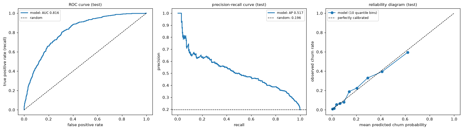
Test-set ROC and precision-recall curves, and the reliability diagram. The points follow the diagonal closely, so a predicted 30% means roughly 30%.
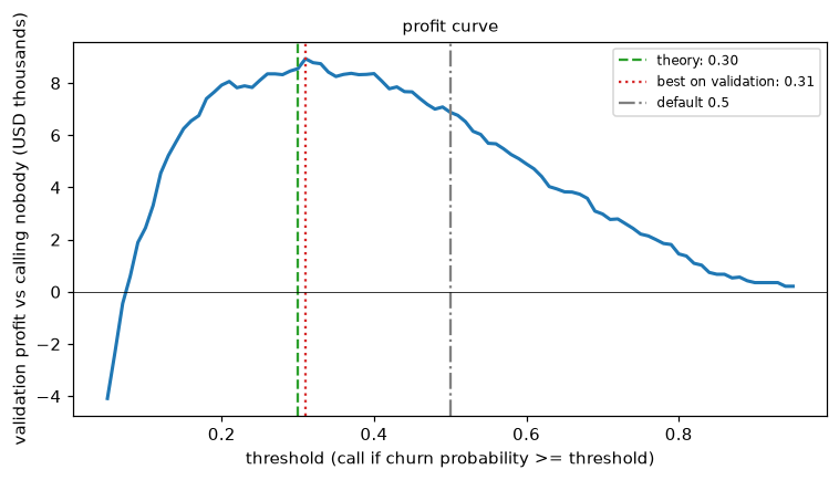
Validation profit by threshold. The curve has a broad peak around the theoretical threshold of 0.3; the default 0.5 leaves a large share of the profit on the table.
Part F: Matching scikit-learn
scikit-learn's LogisticRegression minimizes \(C\sum_i \ell_i + \frac{1}{2}\lVert\mathbf{w}\rVert^2\) (without penalizing the intercept). Dividing by \(Cn\) gives \(\frac{1}{n}\sum_i \ell_i + \frac{1}{2Cn}\lVert\mathbf{w}\rVert^2\), which is our objective when \(\lambda = \frac{1}{Cn}\), so \(C = \frac{1}{\lambda n}\) with \(n\) the number of training rows.
from sklearn.compose import ColumnTransformer
from sklearn.impute import SimpleImputer
from sklearn.linear_model import LogisticRegression
from sklearn.metrics import roc_auc_score, average_precision_score, brier_score_loss, log_loss
from sklearn.model_selection import cross_val_score
from sklearn.pipeline import Pipeline, make_pipeline
from sklearn.preprocessing import OneHotEncoder, StandardScaler
from sklearn.calibration import calibration_curve


def sk_pipeline(C):
    pre = ColumnTransformer([
        ("num", make_pipeline(SimpleImputer(strategy="median", add_indicator=True), StandardScaler()), NUM),
        ("cat", OneHotEncoder(drop="first"), CAT),
    ])
    return Pipeline([("pre", pre), ("clf", LogisticRegression(C=C, tol=1e-12, max_iter=10_000))])


C = 1 / (lam * len(y_tr))
sk = sk_pipeline(C).fit(X_tr_df, y_tr)
print(f"lambda = {lam:.1e}  ->  C = {C:.4f}")
print("features match:", np.allclose(sk["pre"].transform(X_te_df), X_te))
w_sk = np.r_[sk["clf"].intercept_, sk["clf"].coef_.ravel()]
p_sk = sk.predict_proba(X_te_df)[:, 1]
print(f"max |coefficient difference|: {np.abs(w_sk - w_hat).max():.1e}")
print(f"max |probability difference|: {np.abs(p_sk - p_te).max():.1e}")

sk_metrics = {"ROC-AUC": roc_auc_score(y_te, p_te), "average precision (PR-AUC)": average_precision_score(y_te, p_te),
              "Brier score": brier_score_loss(y_te, p_te), "log-loss": log_loss(y_te, p_te)}
for k_ in test_metrics:
    print(f"{k_:>27}: ours {test_metrics[k_]:.6f}   sklearn {sk_metrics[k_]:.6f}")
frac_sk, mean_sk = calibration_curve(y_te, p_te, n_bins=10, strategy="quantile")
print("calibration bins match:", np.allclose(frac_sk, frac_pos) and np.allclose(mean_sk, mean_pred))

print("\ncross-validated log-loss with our folds, ours vs sklearn:")
for l in [1e-4, 1e-2, 1e-1]:
    s = -cross_val_score(sk_pipeline(1 / (l * len(folds[0][0]))), X_tr_df, y_tr, cv=folds, scoring="neg_log_loss")
    print(f"lambda = {l:.0e}: ours {cv[l][0]:.5f}   sklearn {s.mean():.5f}")
lambda = 3.2e-04  ->  C = 0.5270
features match: True
max |coefficient difference|: 1.4e-06
max |probability difference|: 3.9e-07
                    ROC-AUC: ours 0.816238   sklearn 0.816238
 average precision (PR-AUC): ours 0.516636   sklearn 0.516636
                Brier score: ours 0.124038   sklearn 0.124038
                   log-loss: ours 0.387914   sklearn 0.387914
calibration bins match: True

cross-validated log-loss with our folds, ours vs sklearn:
lambda = 1e-04: ours 0.36803   sklearn 0.36803
lambda = 1e-02: ours 0.37283   sklearn 0.37283
lambda = 1e-01: ours 0.40309   sklearn 0.40309
Everything agrees: the feature matrices, the coefficients and probabilities (to the solvers' tolerance), every test metric, the calibration bins, and the cross-validated log-loss for each \(\lambda\). Note one subtlety in the last check: inside cross-validation, each fit sees only the fold's training rows, so C must be computed with that \(n\), not the full training size.
Which features matter?
coefs = pd.Series(w_hat[1:], index=prep.names_).sort_values(key=np.abs, ascending=False)
print(coefs.round(3).head(8).to_string())
contract=two-year                 -1.887
contract=one-year                 -0.978
tenure_months                     -0.839
satisfaction_score                -0.487
autopay=yes                       -0.471
monthly_charges                    0.465
payment_method=electronic check    0.445
days_since_last_login              0.398
Because the numeric features are standardized, their coefficients are log-odds changes per standard deviation; the categorical ones are log-odds differences from the dropped reference level (month-to-month for contract, bank transfer for payment_method, dsl for internet_service). The largest effects are the contract type and tenure. These are associations, not causal effects: moving a customer onto a contract might not reduce their churn risk as much as the coefficient suggests, because customers who choose contracts differ in other ways. That's a question for an experiment, not this model.
The one-page summary for Priya
called = int((p_te >= t_best).sum())
saved = profit(y_te, p_te, t_best)
print(f"Call customers whose predicted churn probability is at least {t_best:.0%}: "
      f"{called} of {len(y_te)} test customers ({called / len(y_te):.0%}).")
print(f"Expected profit on these {len(y_te)} customers: USD {saved:,.0f}, versus USD 0 for calling nobody and "
      f"USD {profit(y_te, p_te, 0.0):,.0f} for calling everybody.")
Call customers whose predicted churn probability is at least 31%: 467 of 2000 test customers (23%).
Expected profit on these 2000 customers: USD 7,990, versus USD 0 for calling nobody and USD -20,800 for calling everybody.
Recommendation. Each month, call the customers whose predicted churn probability is at least the chosen threshold, about a quarter of the base. On the 2,000 held-out test customers, this policy is worth about USD 8,000 a month compared with calling nobody, about USD 2,500 more than using a 50% cutoff, while calling everybody would lose about USD 21,000. The threshold follows from the economics: an offer pays for itself when the churn probability exceeds USD 30 / (40% × USD 250) = 30%.
How good is the model? It ranks well: a random churner gets a higher score than a random non-churner about 82% of the time (ROC-AUC), and among the customers it flags, 47% churn, more than twice the 20% base rate, while it catches 56% of all churners. Its probabilities are calibrated: across ten groups of test customers, the predicted and observed churn rates differ by at most about 5 percentage points, so Finance can use them for forecasts.
What drives churn? Month-to-month contracts, short tenure, low satisfaction scores, and high monthly charges are associated with higher churn; two-year contracts and autopay with lower. These are correlations; test interventions (such as contract incentives) with an A/B test before acting on them.
Why trust it? The model was built from first principles, every metric was computed by hand, and a standard library (scikit-learn) reproduces it to many decimal places. It was evaluated once on customers it had never seen.
What to take away
- Preprocessing is part of the model: fit it on training data, refit it inside each CV fold, and add missing indicators when missingness carries information.
- The gradient check, the curvature-based step size, and the comparison with scikit-learn are cheap, and together they make the from-scratch model trustworthy.
- Regularization strength barely mattered here because \(n\) is large relative to \(d\); cross-validation told us so rather than us assuming it.
- The business threshold (about 0.3) differs sharply from the default 0.5, and choosing it from costs is worth far more money here than tuning the regularization strength.
- Calibration is what lets the probabilities be used as numbers; check it with a reliability diagram, not just AUC.