Transfer Learning

Level 7 · Chapter 6 · ⏱️ ~75 min read · Prerequisites: Convolutional neural networks, Embeddings and NLP basics, The training loop

Most real deep learning projects don't start from random weights. They start from a model someone else trained on a large dataset and adapt it. This chapter explains why pretrained models transfer, the two main strategies (feature extraction and fine-tuning), how to freeze and unfreeze layers (including a batch-norm trap), discriminative learning rates, and domain shift. You'll run a complete, honest transfer experiment on a CPU (pretrain a CNN on five FashionMNIST classes, transfer it to the other five with a handful of labels, and compare training from scratch, frozen features, and fine-tuning), see a domain shift break a model and a two-line fix repair it, and then learn the standard workflows for torchvision pretrained models and the Hugging Face ecosystem.

Why it matters

Sam's team at a regional hospital network wanted to flag chest X-rays that needed urgent review. They had 2,000 labeled images, carefully annotated by radiologists over six months. Their first model, a CNN trained from scratch, reached a validation AUC that looked promising and then collapsed on the next month's images. Two thousand images were simply not enough to learn what edges, textures, and shapes look like and what pneumonia looks like.

The second attempt took a ResNet pretrained on ImageNet's 1.2 million everyday photographs (dogs, cars, teapots) and fine-tuned it on the same 2,000 X-rays. It trained in an afternoon and was clearly better, and more stable from month to month. Nothing in ImageNet is an X-ray, but the early layers had already learned general visual building blocks, and the team's scarce labels went into learning the medical part.

The third lesson came later. The model was deployed at a second hospital whose scanners produced brighter, lower-contrast images, and its accuracy dropped sharply, with no error message. The inputs had shifted. Knowing how to recognize and handle that domain shift turned out to be as important as the transfer itself. This chapter covers all three lessons.

Concepts

Why pretrained features transfer

A CNN trained on a large, varied dataset learns a hierarchy of features, as you saw in the CNN chapter. First-layer filters become edge, color, and blob detectors. Middle layers combine them into textures and simple parts. The last layers respond to object parts and whole objects specific to the training classes.

Yosinski et al. (2014) measured how this generality changes with depth. They split ImageNet's classes into two halves, trained a network on one half, and transferred the first \(n\) layers to a network for the other half. Early-layer features transferred almost perfectly: they're general, useful for almost any image task. Later-layer features were increasingly specific to their original classes, and transferring them helped less, especially between dissimilar tasks. Even so, transferred features with fine-tuning beat random initialization, and the boost persisted after extensive fine-tuning.

There are three ways to see why transfer helps:

• Representation. A model pretrained on millions of images has already learned features that a small dataset could never teach. Your labels go toward combining them, a much easier problem.
• Initialization. Fine-tuning starts gradient descent from a point that's already good, in a region of weight space where the loss surface is well behaved, instead of from random noise.
• Regularization. Training briefly with a small learning rate from pretrained weights \(\theta_0\) keeps the solution near \(\theta_0\). That acts like a prior centered at the pretrained weights. You can make it explicit: the L2-SP penalty (Li, Grandvalet, and Davoine, 2018) adds \(\frac{\alpha}{2}\lVert\theta - \theta_0\rVert^2\) to the loss, which is weight decay toward the pretrained weights instead of toward zero. With few labels, this prior is what prevents overfitting.

The same idea drives modern NLP: a language model pretrained on huge amounts of text learns syntax, facts, and word meanings (the embeddings of the previous chapter, but contextual), and you fine-tune it on your task. "Pretrain once at great expense, adapt cheaply many times" is how most of deep learning is now practiced.

Feature extraction versus fine-tuning

Split a pretrained network into a backbone (everything up to the last hidden layer) and a head (the final classifier). You always replace the head, since your classes differ from the original ones. The question is what to do with the backbone.

Feature extraction freezes the backbone and trains only a new head. The backbone becomes a fixed function \(\phi(\mathbf{x})\) that maps each input to a feature vector, and the head is a linear model on those features:

\[ \hat{y} = \operatorname{softmax}\left(W\phi(\mathbf{x}) + \mathbf{b}\right). \]

That's multinomial logistic regression on the features, the model from Logistic regression, and it's also called a linear probe. It's fast (compute the features once, then train a tiny model), needs very little data, and can't overfit the backbone because the backbone doesn't change. Its limit is that the features stay tuned to the original task.

Fine-tuning initializes the backbone with the pretrained weights and trains everything, usually with a smaller learning rate for the backbone than for the head. It adapts the features to your task and usually gives the best accuracy when you have enough labels, at the cost of more compute and a higher risk of overfitting or of catastrophic forgetting (destroying useful pretrained features with large early updates).

A rough guide, from the CS231n course notes and common practice:

	Target data similar to pretraining data	Target data quite different
Little labeled data	Feature extraction (linear probe on the last layer)	Probe or fine-tune from earlier layers, which are more general; expect smaller gains
Lots of labeled data	Fine-tune the whole network	Fine-tune the whole network; training from scratch becomes competitive

Treat it as a starting point, not a rule. Experiments like the one below are cheap: run them.

Freezing and unfreezing

Freezing a parameter means not updating it: set p.requires_grad_(False), so autograd computes no gradient for it, and give the optimizer only the parameters that are still trainable. Freezing the backbone also saves memory and time, because no activations need to be kept for the backward pass through it.

There's one trap. Batch norm layers have buffers, not just parameters. In train mode, a batch-norm layer keeps updating its running mean and variance from every batch it sees, even if its weight and bias are frozen. So a "frozen" backbone in train mode silently changes, and its statistics drift toward your small dataset. For true feature extraction, put the frozen part in eval mode (backbone.eval()) after each call to model.train(). (Whether to let batch-norm statistics adapt during fine-tuning is a real choice; with very small batches, keeping them frozen is usually safer.)

Gradual unfreezing (popularized by ULMFiT, Howard and Ruder, 2018) combines the two strategies: train the new head with the backbone frozen first, so that a randomly initialized head doesn't send large, noisy gradients into good pretrained weights; then unfreeze the top block, then the next, and so on, fine-tuning more of the network as training proceeds.

Discriminative learning rates

Different layers need different amounts of change. Early layers hold general features that are already good, while the head starts from scratch. Discriminative learning rates (also called layer-wise learning rates) give each part of the network its own rate: small for early layers, larger for later ones, largest for the head. ULMFiT used \(\eta_{l-1} = \eta_l / 2.6\) from each layer group to the one below it, a heuristic.

In PyTorch, this is just parameter groups: the optimizer accepts a list of dictionaries, each with its own parameters and options.

optimizer = torch.optim.AdamW([
    {"params": model.backbone.parameters(), "lr": 1e-4},
    {"params": model.head.parameters(), "lr": 1e-3},
], weight_decay=0.01)

Each group can also have its own weight decay, momentum, and schedule (schedulers scale every group's rate). A related trick is a short warmup at the start of fine-tuning, which keeps the first, noisiest updates small.

Domain shift

A model learns \(p(y \mid \mathbf{x})\) from data drawn from a source distribution, and it's deployed on a target distribution. When they differ, you have domain shift, also called distribution shift or dataset shift. You met its production face, drift, in ML in production. The standard taxonomy:

• Covariate shift: the input distribution \(p(\mathbf{x})\) changes while \(p(y \mid \mathbf{x})\) stays the same. Different scanners, cameras, lighting, microphones, or writing styles. The X-rays in the story.
• Label shift (prior shift): the class frequencies \(p(y)\) change. A disease is rarer at one hospital than another.
• Concept shift: the relationship \(p(y \mid \mathbf{x})\) itself changes. What counts as "spam" evolves.

Deep networks can be strikingly brittle under covariate shift, because they exploit any statistical regularity in their training data, including ones that humans consider irrelevant: brightness, texture, background, the scanner's typeface in an X-ray corner. Remedies, roughly from cheapest to most involved:

1. Detect it. Monitor input statistics and prediction confidence in production; compare with the training data.
2. Augment for it. If you can anticipate the shift (brightness, blur, crops), augment with it during training.
3. Recalibrate normalization. AdaBN (Li et al., 2016) recomputes batch-norm statistics on unlabeled target-domain data, with no labels and no gradient steps. It works when the shift is mostly in low-level statistics, as you'll see below.
4. Fine-tune on a few labeled target examples. This is transfer learning again, with the source model as the pretrained model.
5. Domain adaptation methods that learn features which can't distinguish source from target, using unlabeled target data. They're beyond this chapter.

Pretrained model zoos

You rarely pretrain yourself. Pretrained weights come from:

• torchvision.models: ResNets, EfficientNets, ConvNeXt, vision transformers, detection and segmentation models, each with weights trained on ImageNet or COCO. Each weights object carries its own preprocessing (weights.transforms()), because inputs must be preprocessed exactly as during pretraining: the same resolution, the same normalization mean and standard deviation, the same channel order.
• timm (PyTorch Image Models): a library with hundreds of image architectures and pretrained weights.
• The Hugging Face Hub: hundreds of thousands of models for text, vision, audio, and multimodal tasks, loaded with the transformers library.

Check every pretrained model's license and its model card (documentation of training data, intended use, and known limitations) before building on it. The training data of a pretrained model is part of your system: its biases and gaps become yours.

In practice

Setting up the experiment

The demonstration uses FashionMNIST in two halves. The source task is classes 0–4 (T-shirt/top, Trouser, Pullover, Dress, Coat), with all 30,000 training images. The target task is classes 5–9 (Sandal, Shirt, Sneaker, Bag, Ankle boot), with only a handful of labels per class. The target test set is the 5,000 official test images of classes 5–9. The source classes are mostly upper-body garments and the target classes mostly footwear and bags, so this is a transfer between related but clearly different domains.

import copy
import time

import numpy as np
import torch
import torch.nn as nn
import torch.nn.functional as F
from sklearn.linear_model import LogisticRegression
from torchvision import datasets

torch.set_num_threads(4)

train_full = datasets.FashionMNIST("data", train=True, download=True)
test_full = datasets.FashionMNIST("data", train=False, download=True)
MEAN, STD = 0.2860, 0.3530

def prep(images):
    return ((images.float() / 255 - MEAN) / STD).unsqueeze(1)

def half(ds, first):
    """Classes first..first+4, relabeled 0..4."""
    m = (ds.targets >= first) & (ds.targets < first + 5)
    return prep(ds.data[m]), ds.targets[m] - first

X_src, y_src = half(train_full, 0)
X_src_test, y_src_test = half(test_full, 0)
X_tgt, y_tgt = half(train_full, 5)
X_tgt_test, y_tgt_test = half(test_full, 5)
print("source classes:", train_full.classes[:5])
print("target classes:", train_full.classes[5:])
print(f"source train {len(y_src):,} | target pool {len(y_tgt):,} | target test {len(y_tgt_test):,}")

source classes: ['T-shirt/top', 'Trouser', 'Pullover', 'Dress', 'Coat']
target classes: ['Sandal', 'Shirt', 'Sneaker', 'Bag', 'Ankle boot']
source train 30,000 | target pool 30,000 | target test 5,000

The model is a small CNN, split explicitly into a backbone and a head:

def conv_block(c_in, c_out):
    return nn.Sequential(nn.Conv2d(c_in, c_out, 3, padding=1, bias=False), nn.BatchNorm2d(c_out),
                         nn.ReLU(), nn.MaxPool2d(2))

class Net(nn.Module):
    def __init__(self, n_classes=5):
        super().__init__()
        self.backbone = nn.Sequential(conv_block(1, 32), conv_block(32, 64), conv_block(64, 128),
                                      nn.AdaptiveAvgPool2d(1), nn.Flatten())       # -> 128 features
        self.head = nn.Linear(128, n_classes)

    def forward(self, x):
        return self.head(self.backbone(x))

def train_steps(model, X, y, steps, param_groups, batch_size=64, seed=0, frozen_bn=None):
    """Adam on random minibatches drawn from (X, y)."""
    gen = torch.Generator().manual_seed(seed)
    opt = torch.optim.Adam(param_groups)
    for _ in range(steps):
        model.train()
        if frozen_bn is not None:
            frozen_bn.eval()                               # keep frozen batch-norm statistics fixed
        idx = torch.randint(0, len(y), (min(batch_size, len(y)),), generator=gen)
        loss = F.cross_entropy(model(X[idx]), y[idx])
        opt.zero_grad()
        loss.backward()
        opt.step()
    return model

@torch.no_grad()
def accuracy(model, X, y):
    model.eval()
    return sum((model(X[i:i + 1000]).argmax(1) == y[i:i + 1000]).sum().item() for i in range(0, len(y), 1000)) / len(y)

torch.manual_seed(0)
t0 = time.time()
source = Net()
source = train_steps(source, X_src, y_src, steps=2 * len(y_src) // 128,
                     param_groups=[{"params": source.parameters(), "lr": 2e-3}], batch_size=128)
print(f"pretrained on the source task in {time.time() - t0:.0f}s: source test accuracy {accuracy(source, X_src_test, y_src_test):.3f}")
print("parameters:", sum(p.numel() for p in source.parameters()))

pretrained on the source task in 30s: source test accuracy 0.898
parameters: 93541

Two epochs on the source task give 90% accuracy on its five classes. That model is our "pretrained network". It's tiny next to an ImageNet model, but the mechanics are identical.

Pretrained features versus random features

First, do the source model's features carry information about the target classes, which it never saw? Freeze both the pretrained backbone and a randomly initialized one, extract 128-dimensional features for every target image, and fit a logistic-regression probe with 30 labels per class:

@torch.no_grad()
def features(backbone, X):
    backbone.eval()
    return torch.cat([backbone(X[i:i + 1000]) for i in range(0, len(X), 1000)]).numpy()

def sample_labels(n_per_class, seed):
    gen = torch.Generator().manual_seed(seed)
    idx = [torch.nonzero(y_tgt == c).view(-1)[torch.randperm(int((y_tgt == c).sum()), generator=gen)[:n_per_class]]
           for c in range(5)]
    return torch.cat(idx)

torch.manual_seed(0)
random_backbone = Net().backbone
F_pre_test, F_rand_test = features(source.backbone, X_tgt_test), features(random_backbone, X_tgt_test)
idx = sample_labels(30, seed=0)
for name, bb, F_test in [("pretrained", source.backbone, F_pre_test), ("random", random_backbone, F_rand_test)]:
    probe = LogisticRegression(max_iter=3000).fit(features(bb, X_tgt[idx]), y_tgt[idx].numpy())
    print(f"linear probe on {name:10s} features, 30 labels/class: {(probe.predict(F_test) == y_tgt_test.numpy()).mean():.3f}")

linear probe on pretrained features, 30 labels/class: 0.904
linear probe on random     features, 30 labels/class: 0.756

The pretrained features, learned only from tops, trousers, and coats, separate sandals, sneakers, bags, and boots far better than random features do. Edges, outlines, and textures are useful everywhere.

The comparison: scratch, frozen features, and fine-tuning

Now the main experiment. For several label budgets (3, 10, and 30 labeled images per class), and two random draws of the labeled images each, compare:

• From scratch: a new Net trained on the few labels (Adam, learning rate \(10^{-3}\)).
• Frozen features (linear probe): logistic regression on the pretrained backbone's features.
• Fine-tuning: the pretrained backbone plus a new head, all trained, with discriminative learning rates (\(10^{-4}\) for the backbone, \(10^{-3}\) for the head).

Every network gets the same 150 training steps.

budgets, seeds = [3, 10, 30], [0, 1]
results = {m: {n: [] for n in budgets} for m in ["from scratch", "frozen features (probe)", "fine-tuning"]}
t0 = time.time()
for n in budgets:
    for seed in seeds:
        idx = sample_labels(n, seed)
        X, y = X_tgt[idx], y_tgt[idx]

        torch.manual_seed(seed)
        scratch = Net()
        train_steps(scratch, X, y, 150, [{"params": scratch.parameters(), "lr": 1e-3}], seed=seed)
        results["from scratch"][n].append(accuracy(scratch, X_tgt_test, y_tgt_test))

        probe = LogisticRegression(max_iter=3000).fit(features(source.backbone, X), y.numpy())
        results["frozen features (probe)"][n].append((probe.predict(F_pre_test) == y_tgt_test.numpy()).mean())

        torch.manual_seed(seed)
        ft = Net()
        ft.backbone = copy.deepcopy(source.backbone)                       # pretrained weights, new head
        train_steps(ft, X, y, 150, [{"params": ft.backbone.parameters(), "lr": 1e-4},
                                    {"params": ft.head.parameters(), "lr": 1e-3}], seed=seed)
        results["fine-tuning"][n].append(accuracy(ft, X_tgt_test, y_tgt_test))

print(f"({time.time() - t0:.0f}s)  target test accuracy, mean over {len(seeds)} draws of the labeled images")
print(f"{'labels per class':26s}" + "".join(f"{n:>8d}" for n in budgets))
for method, by_n in results.items():
    print(f"{method:26s}" + "".join(f"{np.mean(by_n[n]):8.3f}" for n in budgets))

(50s)  target test accuracy, mean over 2 draws of the labeled images
labels per class                 3      10      30
from scratch                 0.704   0.852   0.903
frozen features (probe)      0.642   0.823   0.883
fine-tuning                  0.716   0.853   0.894

import matplotlib.pyplot as plt

fig, ax = plt.subplots(figsize=(7.5, 4.2))
for method, marker in zip(results, ["o", "s", "^"]):
    means = [np.mean(results[method][n]) for n in budgets]
    ax.plot(budgets, means, marker=marker, label=method)
    for n in budgets:
        ax.scatter([n] * len(seeds), results[method][n], marker=marker, alpha=0.3, s=15)
ax.set(xscale="log", xticks=budgets, xticklabels=[str(n) for n in budgets], xlabel="labeled images per target class (log scale)",
       ylabel="target test accuracy", title="Transfer from classes 0-4 to classes 5-9")
ax.grid(alpha=0.3)
ax.legend()
plt.show()

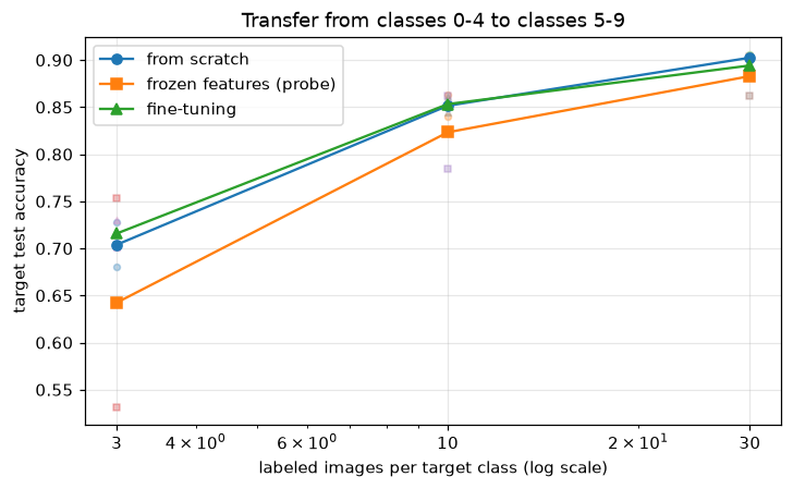Lines are means over two draws of the labeled images; faint points are the individual runs. With these related-but-different domains, the methods are close.

This is an honest result, and it's more instructive than a dramatic one:

• Fine-tuning edges out training from scratch only when labels are scarcest: by about a point at 3 labels per class. At 10 they're tied, and at 30 scratch is slightly ahead. All of these differences are about the size of the spread between the two draws. The pretrained starting point helps a little, not a lot.
• Frozen features are the worst of the three here, even though they're far better than random features. The source model's last-layer features specialize in what distinguishes T-shirts from pullovers and coats; they're less suited to telling sandals from sneakers, which is exactly Yosinski's specificity effect, and exactly the "quite different data" column of the table in the Concepts section.
• Training from scratch is strong because this target task is easy (sandals, sneakers, bags, boots, and shirts look very different) and a small CNN's architecture already encodes a lot (locality, weight sharing). With 30 labels per class, it reaches 90%.

Why do real-world transfers usually look far better than this? Three differences. ImageNet pretraining sees 1.2 million images of 1,000 diverse classes, so its features are far more general than features from 30,000 images of five garment types. Real target tasks are usually harder than separating shoes from bags, so scratch training needs much more data. And modern backbones are much deeper, so there's much more to learn from scratch. The mechanics you just used are the same ones you'd use with a pretrained ResNet; the size of the benefit depends on how much, and how relevant, the pretraining was. Measure it, don't assume it.

Common mistake: comparing on one random draw

With 3 labels per class, which 15 images you happen to label moves accuracy by several points (look at the faint points in the figure). A single run can make either method look better. Average over several draws, and over seeds, before concluding, as in the training loop.

Freezing correctly, and the batch-norm trap

To freeze the backbone, turn off its gradients and give the optimizer only the head. Then check what actually stays fixed:

model = Net()
model.backbone = copy.deepcopy(source.backbone)
for p in model.backbone.parameters():
    p.requires_grad_(False)
trainable = [n for n, p in model.named_parameters() if p.requires_grad]
print("trainable:", trainable, "| frozen tensors:", sum(not p.requires_grad for p in model.parameters()))

bn = model.backbone[0][1]                                   # first batch-norm layer
before = bn.running_mean.clone()
model.train()                                               # the usual call at the top of an epoch...
with torch.no_grad():
    model(X_tgt[:64])
print("frozen BN running mean changed in train mode:", not torch.equal(before, bn.running_mean))

bn.running_mean.copy_(before)
model.train()
model.backbone.eval()                                       # ...followed by this, for true feature extraction
with torch.no_grad():
    model(X_tgt[:64])
print("after backbone.eval():                    ", not torch.equal(before, bn.running_mean))

trainable: ['head.weight', 'head.bias'] | frozen tensors: 9
frozen BN running mean changed in train mode: True
after backbone.eval():                     False

requires_grad_(False) froze the weights but not the running statistics, which changed on a single forward pass in train mode. Calling backbone.eval() after model.train() keeps them fixed. (The frozen_bn argument of train_steps does exactly that.)

Discriminative learning rates and gradual unfreezing

Parameter groups let you give each depth its own learning rate. Here is a ULMFiT-style geometric schedule over the three convolutional blocks and the head, with each lower group's rate 2.6 times smaller:

model = Net()
model.backbone = copy.deepcopy(source.backbone)
head_lr = 1e-3
groups = [{"params": model.head.parameters(), "lr": head_lr, "name": "head"}]
for depth, block in enumerate(reversed(list(model.backbone[:3]))):
    groups.append({"params": block.parameters(), "lr": head_lr / 2.6 ** (depth + 1), "name": f"conv block {3 - depth}"})
opt = torch.optim.AdamW(groups, weight_decay=1e-4)
for g in opt.param_groups:
    print(f"{g['name']:12s} lr {g['lr']:.2e}  ({sum(p.numel() for p in g['params']):,} parameters)")

head         lr 1.00e-03  (645 parameters)
conv block 3 lr 3.85e-04  (73,984 parameters)
conv block 2 lr 1.48e-04  (18,560 parameters)
conv block 1 lr 5.69e-05  (352 parameters)

Gradual unfreezing is a loop over stages: freeze everything except the head, train, unfreeze the next block down, add it to the optimizer, train again. Exercise 4 asks you to implement it and compare.

Domain shift: a model that breaks, and two fixes

Back to the second hospital. Simulate its brighter, low-contrast scanner by transforming the source test images: each pixel value \(p \in [0, 1]\) becomes \(0.4p + 0.5\). The images are still perfectly recognizable to a person.

def faded(X):
    """Simulate a different camera: compress contrast and brighten, in pixel space, then renormalize."""
    pixels = X * STD + MEAN
    return (0.4 * pixels + 0.5 - MEAN) / STD

print(f"source model, original test images: {accuracy(source, X_src_test, y_src_test):.3f}")
print(f"source model, faded test images:    {accuracy(source, faded(X_src_test), y_src_test):.3f}  (chance = 0.200)")

source model, original test images: 0.898
source model, faded test images:    0.200  (chance = 0.200)

Accuracy drops from 90% to exactly chance. The model sees inputs whose statistics it never saw, and its first batch-norm layer normalizes them with the wrong mean and variance, so every later layer receives activations far outside its training range. Nothing crashes; it just answers wrong.

Fix 1: AdaBN, which needs no labels. Reset the batch-norm running statistics and recompute them from unlabeled images of the new domain, by running forward passes in train mode without gradients:

adapted = copy.deepcopy(source)
for m in adapted.modules():
    if isinstance(m, nn.BatchNorm2d):
        m.reset_running_stats()
        m.momentum = None                     # None = a cumulative average over all batches seen
adapted.train()
with torch.no_grad():
    for i in range(0, 5000, 500):             # 5,000 UNLABELED images from the new "scanner"
        adapted(faded(X_src[i:i + 500]))
print(f"AdaBN model, faded test images:     {accuracy(adapted, faded(X_src_test), y_src_test):.3f}")
print(f"AdaBN model, original test images:  {accuracy(adapted, X_src_test, y_src_test):.3f}")

AdaBN model, faded test images:     0.893
AdaBN model, original test images:  0.305

Recomputing the statistics restores 89% on the faded images, without a single label or gradient step. The adapted model now fails on the original images instead: batch-norm statistics are domain-specific, so each domain needs its own. This shift was an affine change of pixel values, which batch normalization undoes almost exactly, so it's a best case for AdaBN. Real shifts (different anatomy, different noise, different objects) are rarely so simple.

Fix 2: fine-tune on a few labeled target examples, which handles shifts that normalization alone can't:

idx = torch.randperm(len(y_src), generator=torch.Generator().manual_seed(0))[:100]   # 100 labeled faded images
torch.manual_seed(0)
tuned = copy.deepcopy(source)
train_steps(tuned, faded(X_src[idx]), y_src[idx], 100,
            [{"params": tuned.backbone.parameters(), "lr": 1e-4}, {"params": tuned.head.parameters(), "lr": 1e-3}])
print(f"fine-tuned on 100 labeled faded images: {accuracy(tuned, faded(X_src_test), y_src_test):.3f}")

fine-tuned on 100 labeled faded images: 0.908

With only 100 labeled images from the new domain, fine-tuning recovers to 91%, slightly better than AdaBN: transfer learning from the old domain to the new one. In practice you'd combine both fixes, plus augmentation (random brightness and contrast during training) so the next scanner doesn't break the model at all.

Common mistake: silent domain shift

Domain shift doesn't raise errors. The model above returned confident-looking predictions on faded images while being right only at chance level. Monitor input statistics (mean pixel intensity here would have exposed it immediately) and the distribution of predicted classes in production, as in ML in production.

Fine-tuning a torchvision ResNet-18

With a pretrained ImageNet model, the workflow is the same, plus matching the pretraining preprocessing. The weights need a download (about 45 MB), so the code below isn't run on this page. It fine-tunes ResNet-18 on FashionMNIST, which means converting the \(28 \times 28\) grayscale images to 3-channel images at the resolution the model expects.

import torch
import torch.nn as nn
from torch.utils.data import DataLoader
from torchvision import datasets
from torchvision.models import ResNet18_Weights, resnet18
from torchvision.transforms import v2

weights = ResNet18_Weights.DEFAULT                     # ImageNet-1k weights
model = resnet18(weights=weights)                      # downloads to ~/.cache/torch on first use
print(weights.transforms())                            # the preprocessing these weights expect

preprocess = v2.Compose([
    v2.ToImage(), v2.ToDtype(torch.float32, scale=True),
    v2.Grayscale(num_output_channels=3),               # 1 channel -> 3 identical channels
    v2.Resize(112),                                     # smaller than 224 to save compute; still works
    v2.Normalize(mean=[0.485, 0.456, 0.406], std=[0.229, 0.224, 0.225]),   # ImageNet statistics
])
train_ds = datasets.FashionMNIST("data", train=True, download=True, transform=preprocess)
test_ds = datasets.FashionMNIST("data", train=False, download=True, transform=preprocess)

model.fc = nn.Linear(model.fc.in_features, 10)         # new head: 512 -> 10

# Stage 1: feature extraction (head only, backbone frozen and in eval mode)
for name, p in model.named_parameters():
    p.requires_grad = name.startswith("fc.")
# Stage 2: fine-tune everything with discriminative learning rates
optimizer = torch.optim.AdamW([
    {"params": [p for n, p in model.named_parameters() if n.startswith(("conv1", "bn1", "layer1", "layer2"))], "lr": 1e-5},
    {"params": [p for n, p in model.named_parameters() if n.startswith(("layer3", "layer4"))], "lr": 1e-4},
    {"params": model.fc.parameters(), "lr": 1e-3},
], weight_decay=1e-4)
# ...then the training loop from Chapter 2, on a GPU if you have one.

Illustrative output of the print(weights.transforms()) line (not run on this page):

ImageClassification(
    crop_size=[224]
    resize_size=[256]
    mean=[0.485, 0.456, 0.406]
    std=[0.229, 0.224, 0.225]
    interpolation=InterpolationMode.BILINEAR
)

Illustrative results (not run on this page; your numbers will vary): head-only training reaches the mid-80s percent on FashionMNIST in one epoch, and full fine-tuning for a couple of epochs reaches the low-to-mid 90s, at a cost of minutes per epoch on a GPU and roughly an hour per epoch on a laptop CPU at this resolution. The capstone gets above 90% with a model 100 times smaller trained from scratch, because FashionMNIST is small, simple, and plentiful. Transfer pays off when your images are closer to natural photographs and your labels are scarce.

Hugging Face basics

For text (and increasingly for everything else), the Hugging Face ecosystem is the standard source of pretrained models. Three libraries do most of the work: transformers (models and tokenizers), datasets (dataset loading and processing), and the Hub (hosting, versioning, and model cards). transformers isn't installed in this handbook's reference environment, and its models must be downloaded, so the code below isn't run on this page; the outputs shown are illustrative.

The highest-level API is the pipeline, which bundles preprocessing, the model, and postprocessing:

from transformers import pipeline

classifier = pipeline("sentiment-analysis", model="distilbert-base-uncased-finetuned-sst-2-english")
print(classifier(["The delivery was fast and the jacket fits perfectly.",
                  "Arrived late and the zipper broke on day one."]))

Illustrative output (not run on this page; your scores will vary slightly):

[{'label': 'POSITIVE', 'score': 0.9998}, {'label': 'NEGATIVE', 'score': 0.9996}]

Underneath, every model comes as a tokenizer plus a model, both loaded with from_pretrained. The tokenizer does the subword tokenization from the previous chapter and returns token IDs and an attention mask (1 for real tokens, 0 for padding):

import torch
from transformers import AutoModelForSequenceClassification, AutoTokenizer

name = "distilbert-base-uncased"
tokenizer = AutoTokenizer.from_pretrained(name)
model = AutoModelForSequenceClassification.from_pretrained(name, num_labels=4)   # new 4-class head

batch = tokenizer(["my refund has not arrived", "the parcel never came"],
                  padding=True, truncation=True, max_length=64, return_tensors="pt")
print(batch["input_ids"].shape, tokenizer.convert_ids_to_tokens(batch["input_ids"][0]))

labels = torch.tensor([0, 1])                          # billing, shipping
out = model(**batch, labels=labels)                    # returns the loss when labels are given
print(out.loss, out.logits.shape)

optimizer = torch.optim.AdamW(model.parameters(), lr=2e-5)   # small LR: fine-tuning a pretrained transformer
out.loss.backward()
optimizer.step()
model.save_pretrained("ticket-router")                 # writes the config and weights
tokenizer.save_pretrained("ticket-router")

Illustrative output (not run on this page; the loss depends on the random head):

torch.Size([2, 8]) ['[CLS]', 'my', 'ref', '##und', 'has', 'not', 'arrived', '[SEP]']
tensor(1.3907, grad_fn=<NllLossBackward0>) torch.Size([2, 4])

A few things to notice. The model is an ordinary nn.Module, so the training loop from Chapter 2 works unchanged. The classification head is newly initialized (the library warns you about it), exactly like replacing fc on a ResNet. The tokenizer added special tokens ([CLS], [SEP]) and split a word into subwords marked ## (the exact split depends on the vocabulary; this one is illustrative). Fine-tuning learning rates for pretrained transformers are small, typically \(10^{-5}\) to \(5 \times 10^{-5}\), because large updates destroy what pretraining learned. The library's Trainer class wraps the loop with mixed precision, logging, and checkpointing. And with the ticket router from the previous chapter in mind: a pretrained tokenizer and model handle "double billed" gracefully, because both the subwords and their meanings were learned from billions of words.

The architectures behind these models (transformers, BERT, GPT) are the subject of Level 8.

Exercises

Exercise 1: Which strategy? (easy)

For each scenario, choose feature extraction, fine-tuning, or training from scratch, and justify it: (a) 300 labeled photos of 5 kinds of houseplant, with an ImageNet-pretrained ResNet; (b) 2 million labeled product photos in 5,000 categories; (c) 500 labeled spectrograms of machine vibrations, with an ImageNet-pretrained model; (d) 50,000 labeled customer emails for intent routing, with a pretrained language model.

Solution

(a) Feature extraction, then perhaps light fine-tuning. Very little data, and plants are well represented in ImageNet-like photos, so pretrained features fit well and a linear probe can't overfit the backbone.

(b) Fine-tune the whole network (or train from scratch). With 2 million labels the risk of overfitting is low, so let all the features adapt. Starting from pretrained weights still converges faster.

(c) Fine-tune, starting cautiously, and compare with a small model trained from scratch. Spectrograms look nothing like photos, so last-layer features transfer poorly; early layers (edges, textures) still help. Try probing or fine-tuning from intermediate layers, with strong regularization and augmentation suited to spectrograms.

(d) Fine-tune the pretrained language model. 50,000 labeled texts is plenty for full fine-tuning with a small learning rate, and pretrained models understand paraphrases a model trained from scratch wouldn't.

Exercise 2: Parameters you train (easy)

For ResNet-18 (11.7 million parameters, of which the final fc layer for 1,000 classes has 513,000), how many parameters are trained (a) in feature extraction with a new 10-class head, and (b) in full fine-tuning with that head? (c) Why does feature extraction also use much less memory per batch?

Solution

(a) Only the new head: \(512 \times 10 + 10 = 5{,}130\) parameters. (b) The backbone (\(11.7\text{M} - 0.513\text{M} \approx 11.18\text{M}\)) plus the new head: about 11.18 million. (c) Training memory is dominated by stored activations for the backward pass, gradients, and optimizer state (two extra copies of each trained parameter for Adam). A frozen backbone needs none of these: no gradients flow into it, so its activations needn't be kept (run it under torch.no_grad()), and the optimizer only tracks 5,130 parameters. You can even precompute the features once and train the head on them, as the chapter's probe does.

Exercise 3: Which layer transfers best? (medium)

Repeat the linear-probe comparison, but probe features from after each convolutional block (global-average-pool the block's output), for the pretrained and the random backbone, with 30 labels per class. How does transferability change with depth?

Solution

@torch.no_grad()
def block_features(backbone, X, depth):
    backbone.eval()
    out = []
    for i in range(0, len(X), 1000):
        h = X[i:i + 1000]
        for k in range(depth):
            h = backbone[k](h)
        out.append(F.adaptive_avg_pool2d(h, 1).flatten(1))
    return torch.cat(out).numpy()

idx = sample_labels(30, seed=0)
for depth in [1, 2, 3]:
    row = []
    for bb in [source.backbone, random_backbone]:
        probe = LogisticRegression(max_iter=3000).fit(block_features(bb, X_tgt[idx], depth), y_tgt[idx].numpy())
        row.append((probe.predict(block_features(bb, X_tgt_test, depth)) == y_tgt_test.numpy()).mean())
    print(f"after block {depth}: pretrained {row[0]:.3f}, random {row[1]:.3f}, gain {row[0] - row[1]:+.3f}")

after block 1: pretrained 0.695, random 0.591, gain +0.105
after block 2: pretrained 0.843, random 0.623, gain +0.220
after block 3: pretrained 0.904, random 0.756, gain +0.148

The pretrained features get more useful with depth, but the gain over random features peaks after block 2 (22 points) and shrinks after block 3 (15 points). The middle block holds the most transferable features; the last block is already partly specialized for distinguishing tops, trousers, and coats. That's Yosinski's generality-to-specificity pattern, visible even in a three-block network. (Random features also improve with depth, because random convolutions followed by pooling are surprisingly good generic features.) In deep networks pretrained on large datasets, the same probe often peaks somewhere before the last layer for distant target tasks. Note that globally pooling block 1's 32 channels throws away almost all spatial information, which is why its probe is weak for both backbones.

Exercise 4: Gradual unfreezing (medium)

Implement two-stage fine-tuning for the 10-labels-per-class budget: 75 steps training only the head (backbone frozen, batch norm in eval mode), then 75 steps training everything with discriminative learning rates. Compare with the chapter's one-stage fine-tuning over the same two draws.

Solution

two_stage = []
for seed in seeds:
    idx = sample_labels(10, seed)
    X, y = X_tgt[idx], y_tgt[idx]
    torch.manual_seed(seed)
    m = Net()
    m.backbone = copy.deepcopy(source.backbone)
    for p in m.backbone.parameters():
        p.requires_grad_(False)
    train_steps(m, X, y, 75, [{"params": m.head.parameters(), "lr": 1e-2}], seed=seed, frozen_bn=m.backbone)
    for p in m.backbone.parameters():
        p.requires_grad_(True)
    train_steps(m, X, y, 75, [{"params": m.backbone.parameters(), "lr": 1e-4},
                               {"params": m.head.parameters(), "lr": 1e-3}], seed=seed)
    two_stage.append(accuracy(m, X_tgt_test, y_tgt_test))
print(f"one-stage fine-tuning {np.mean(results['fine-tuning'][10]):.3f} | two-stage {np.mean(two_stage):.3f}")

one-stage fine-tuning 0.853 | two-stage 0.863

Two-stage is about a point better here, which is within the draw-to-draw spread you saw in the main experiment, so two draws can't settle it. Gradual unfreezing protects pretrained weights from the large, random gradients of a fresh head, which matters most when the backbone is large and valuable (a pretrained transformer or ResNet) and the learning rates are aggressive. With this small backbone and an already small backbone learning rate, there was little to protect. That's typical of tricks like this one: they matter in some regimes and not others, and only an experiment tells you which regime you're in.

Exercise 5: Label shift (hard)

A classifier was trained on balanced classes, but in deployment class 0 is 70% of the inputs and the other four classes 7.5% each. Without retraining, how can you correct the predicted probabilities? Implement it for the source model on a test set resampled to these proportions, and compare accuracy before and after.

Solution

Under pure label shift, \(p(\mathbf{x} \mid y)\) is unchanged, so by Bayes' theorem the target posterior is the source posterior reweighted by the ratio of priors and renormalized:

\[ p_{\text{tgt}}(y \mid \mathbf{x}) \propto p_{\text{src}}(y \mid \mathbf{x})\,\frac{p_{\text{tgt}}(y)}{p_{\text{src}}(y)}. \]

In logit space that's adding \(\log p_{\text{tgt}}(y) - \log p_{\text{src}}(y)\) to each class's logit.

gen = torch.Generator().manual_seed(0)
prior_tgt = torch.tensor([0.70, 0.075, 0.075, 0.075, 0.075])
counts = (prior_tgt * 2000).long()
idx = torch.cat([torch.nonzero(y_src_test == c).view(-1)[torch.randperm(1000, generator=gen)[:counts[c]]] for c in range(5)])
Xs, ys = X_src_test[idx], y_src_test[idx]
with torch.no_grad():
    source.eval()
    logits = source(Xs)
corrected = logits + torch.log(prior_tgt) - torch.log(torch.full((5,), 0.2))
print(f"accuracy before {(logits.argmax(1) == ys).float().mean():.3f}, after prior correction {(corrected.argmax(1) == ys).float().mean():.3f}")

accuracy before 0.939, after prior correction 0.926

The correction made things slightly worse here, and the reason is the important lesson. The formula is exact only if the model's probabilities are calibrated, that is, if they match true frequencies (see Evaluation metrics). A network trained with cross-entropy is typically overconfident, and this one is also already good at the common class (T-shirt/top), so there were few class-0 errors to fix, while the prior boost flipped some correct minority-class predictions to class 0. The fix is to calibrate first, for example with temperature scaling (divide the logits by a scalar \(T\) fitted on validation data), and then apply the prior correction. In practice the target priors are also unknown and must be estimated from unlabeled target predictions (for example with the EM procedure of Saerens et al., 2002, or black-box shift estimation), which again assumes calibration. Prior correction is a tool to test, not a guaranteed win.

Check yourself

1. Why do features from a network pretrained on everyday photos help on X-rays or spectrograms?

   Answer

   Early and middle layers learn general building blocks (edges, textures, simple shapes) that are useful for almost any image. A small dataset can't teach those well, so starting from them lets the labels go toward the task-specific part. The benefit shrinks as the domains get more different, and it's largest for early layers.

2. What's the difference between feature extraction and fine-tuning, and when would you choose each?

   Answer

   Feature extraction freezes the pretrained backbone and trains only a new head (a linear probe on fixed features): cheap, robust with very little data, but the features can't adapt. Fine-tuning trains the whole network starting from the pretrained weights, usually with a smaller learning rate for the backbone: better when you have more data or the target differs from the pretraining data.

3. You froze a backbone with requires_grad_(False), but its behavior still changes during training. Why?

   Answer

   Batch-norm layers update their running mean and variance buffers in train mode regardless of requires_grad. Put the frozen backbone in eval mode after calling model.train().

4. What are discriminative learning rates, and how do you implement them in PyTorch?

   Answer

   Different learning rates for different layers: small for early, general layers, larger for later ones, largest for the new head. In PyTorch, pass the optimizer a list of parameter groups, each a dict with its own params and lr.

5. Why must you use a pretrained model's own preprocessing?

   Answer

   The weights were learned on inputs with a specific resolution, normalization (mean and standard deviation), and channel order. Different preprocessing is itself a domain shift: the first layers see input statistics they were never trained on.

6. Define covariate shift, label shift, and concept shift, with an example of each.

   Answer

   Covariate shift: \(p(\mathbf{x})\) changes, \(p(y \mid \mathbf{x})\) doesn't (a new camera or scanner). Label shift: \(p(y)\) changes, \(p(\mathbf{x} \mid y)\) doesn't (a disease becomes more common). Concept shift: \(p(y \mid \mathbf{x})\) changes (what users consider spam evolves).

7. How does AdaBN adapt a model without labels, and when does it work?

   Answer

   It recomputes batch-norm running statistics on unlabeled target-domain inputs, so each layer's activations are normalized with the new domain's statistics. It works when the shift is mostly in low-level statistics (brightness, contrast, sensor gain); it can't fix shifts in content or in the meaning of features.

8. What does AutoModelForSequenceClassification.from_pretrained(name, num_labels=4) give you, and what's new in it?

   Answer

   A pretrained transformer encoder with a classification head for 4 classes, as an ordinary nn.Module. The encoder weights are pretrained; the classification head is newly initialized and must be trained, typically with a small learning rate (around \(10^{-5}\) to \(5 \times 10^{-5}\)) for the whole model.

Key takeaways

• Pretrained networks transfer because their early and middle layers learn general features; later layers are more specific to the original task.
• Feature extraction (frozen backbone, new head) is cheap and safe with tiny datasets; fine-tuning adapts the features and usually wins with more data or a different domain.
• Freeze with requires_grad_(False), and put frozen batch-norm layers in eval mode. Use parameter groups for discriminative learning rates; consider gradual unfreezing for large, valuable backbones.
• Measure the benefit: in our small experiment, pretrained features beat random ones by about 15 points as a probe, but fine-tuning beat training from scratch by only about a point at the smallest label budget, and not at all with more labels. The size of the gain depends on how much, and how relevant, the pretraining was.
• Domain shift fails silently. Monitor inputs, augment for anticipated shifts, recalibrate batch norm (AdaBN) for low-level shifts, and fine-tune on a few labeled target examples.
• torchvision and Hugging Face models are ordinary nn.Modules: match their preprocessing, replace the head, and reuse your training loop.

Further reading

• Jason Yosinski, Jeff Clune, Yoshua Bengio, and Hod Lipson, "How transferable are features in deep neural networks?" (NeurIPS 2014).
• Jeremy Howard and Sebastian Ruder, "Universal Language Model Fine-tuning for Text Classification" (ACL 2018), which introduced discriminative learning rates and gradual unfreezing.
• Simon Kornblith, Jonathon Shlens, and Quoc V. Le, "Do Better ImageNet Models Transfer Better?" (CVPR 2019).
• Yanghao Li, Naiyan Wang, Jianping Shi, Jiaying Liu, and Xiaodi Hou, "Revisiting Batch Normalization For Practical Domain Adaptation" (2016), the AdaBN paper.
• The Hugging Face course and the torchvision models documentation.

Next

You've completed the chapters of Level 7. Put everything together in the Level 7 capstone: train an image classifier above 90% accuracy with augmentation, tracking, and an error analysis.