Edges and Gradients

Level 1 · Chapter 3 · ⏱️ ~60 min read · Prerequisites: Convolution and filtering

Edges are where the image changes, and change is measured by derivatives. This chapter covers image derivatives and finite differences, the Sobel and Scharr operators, gradient magnitude and direction, the Laplacian, LoG and DoG, and the Canny edge detector built step by step from scratch and checked against OpenCV.

Why it matters

Priya's team flew drones along a concrete bridge to find cracks. The first detector was simple: compute the difference between each pixel and its right neighbor, and flag differences larger than 30. On the first test flight it reported 40,000 "cracks" per image. Concrete has texture, the camera has noise, and a raw pixel difference responds to both just as strongly as to a crack.

Raising the threshold to 80 removed the texture, and most of the cracks with it. The real cracks came out as scattered dots, because a hairline crack is faint in places and its pixel differences dip below any single threshold along its length.

The fix was the Canny edge detector, with each of its steps addressing one of these failures. Smoothing before differentiating suppressed the texture. Non-maximum suppression thinned each crack to a one-pixel line. Hysteresis thresholding, with a high threshold to start a crack and a low one to continue it, followed the faint stretches without admitting the texture. The detector is 40 years old, it's still in OpenCV, and you'll build it yourself in this chapter.

Concepts

What is an edge?

An edge is a place where the image intensity changes sharply over a short distance. Edges matter because they mark the things you care about: object boundaries, surface creases, markings, shadows, and text. A line drawing of a scene, which is roughly what an edge map is, is often enough for a human to recognize everything in it.

Edges in images come from four physical causes: a depth discontinuity (one object in front of another), a change in surface orientation (the crease of a box), a change in reflectance (paint, print, a material boundary), and a change in illumination (a shadow's border). An edge detector can't tell these apart; it only sees intensity change. Interpreting edges is the job of later stages.

Real edges have profiles. A step edge jumps from one level to another. Optics and sensors always blur a little, so in practice you get a ramp. A thin dark line on a light background is two edges close together, a line or ridge profile. A roof edge rises and falls gradually. The first derivative peaks in the middle of a ramp; the second derivative crosses zero there. Those two facts give the two families of edge detectors.

Derivatives by finite differences

For a continuous 1D signal \(f(x)\), the derivative is \(f'(x) = \lim_{h \to 0} \frac{f(x + h) - f(x)}{h}\). An image is sampled on a grid with spacing \(h = 1\) pixel, so you can't take the limit. You approximate the derivative with a finite difference:

• Forward: \(f'(x) \approx f(x + 1) - f(x)\). Kernel \([-1, 1]\) (for correlation), positioned between pixels.
• Backward: \(f'(x) \approx f(x) - f(x - 1)\).
• Central: \(f'(x) \approx \frac{f(x + 1) - f(x - 1)}{2}\). Kernel \(\frac{1}{2}[-1, 0, 1]\), centered on the pixel.

The central difference is more accurate. Expand \(f(x \pm h)\) in a Taylor series:

\[ f(x \pm h) = f(x) \pm h f'(x) + \frac{h^2}{2} f''(x) \pm \frac{h^3}{6} f'''(x) + \dots \]

The forward difference gives \(\frac{f(x + h) - f(x)}{h} = f'(x) + \frac{h}{2} f''(x) + \dots\), an error proportional to \(h\). In the central difference, the even-order terms cancel:

\[ \frac{f(x + h) - f(x - h)}{2h} = f'(x) + \frac{h^2}{6} f'''(x) + \dots, \]

an error proportional to \(h^2\). Halving the spacing cuts the forward error in half but the central error by four. The central difference is also symmetric about the pixel, so it doesn't shift edges by half a pixel. That's why image derivative kernels are built on \([-1, 0, 1]\).

import numpy as np
import cv2
import matplotlib.pyplot as plt
from scipy import ndimage
from skimage import data

x0 = 1.0
for h in [0.5, 0.25, 0.125]:
    fwd = (np.sin(x0 + h) - np.sin(x0)) / h
    cen = (np.sin(x0 + h) - np.sin(x0 - h)) / (2 * h)
    print(f"h={h:<6} forward error {abs(fwd - np.cos(x0)):.5f}   central error {abs(cen - np.cos(x0)):.5f}")

h=0.5    forward error 0.22825   central error 0.02223
h=0.25   forward error 0.11025   central error 0.00561
h=0.125  forward error 0.05393   central error 0.00141

Each halving of \(h\) halves the forward error and quarters the central one, as the Taylor expansion predicts.

Differentiation amplifies noise

Here's the problem Priya hit. Suppose each pixel has independent noise with standard deviation \(\sigma_n\). The central difference \(\frac{1}{2}(f(x+1) - f(x-1))\) subtracts two noisy values, so its noise has standard deviation \(\frac{\sqrt{2}}{2}\sigma_n \approx 0.7\sigma_n\): about the same as the noise in the image. But the signal in a derivative is the slope, which is small except at edges. A gentle edge that rises 30 levels over 10 pixels has a slope of only 3 per pixel, comparable to the derivative of ordinary sensor noise. In the frequency terms of the next chapter: differentiation multiplies each frequency by its frequency, so it boosts exactly the fine-scale wiggles where noise lives.

The cure is to smooth first, then differentiate. And by the associativity of convolution (Chapter 2), smoothing with \(G_\sigma\) and then differentiating equals filtering once with the derivative of a Gaussian:

\[ \frac{\partial}{\partial x}\big(G_\sigma * f\big) = \left(\frac{\partial G_\sigma}{\partial x}\right) * f. \]

The scale \(\sigma\) is a real choice, not a nuisance parameter. Small \(\sigma\) finds fine edges and keeps them well localized, but lets noise through. Large \(\sigma\) suppresses noise and fine texture, finds only large-scale edges, and blurs their positions. There's no universally right value; it depends on the size of the structures you care about.

rng = np.random.default_rng(0)
xs = np.arange(200)
clean = 50 + 100 / (1 + np.exp(-(xs - 100) / 2.0))           # a soft step edge
noisy = clean + rng.normal(0, 5, xs.size)

central = ndimage.correlate1d(noisy, [-0.5, 0, 0.5], mode="nearest")
dog = ndimage.gaussian_filter1d(noisy, sigma=4, order=1, mode="nearest")    # derivative of Gaussian
print("central difference: peak at", np.argmax(central), "| peak/noise", round(central.max() / central[:80].std(), 1))
print("derivative of Gaussian: peak at", np.argmax(dog), "| peak/noise", round(dog.max() / dog[:80].std(), 1))

fig, axes = plt.subplots(1, 3, figsize=(10, 2.6))
axes[0].plot(noisy, lw=0.8); axes[0].set_title("noisy step edge", fontsize=9)
axes[1].plot(central, lw=0.8); axes[1].set_title("central difference", fontsize=9)
axes[2].plot(dog, lw=0.8); axes[2].set_title("derivative of Gaussian, σ = 4", fontsize=9)
plt.tight_layout()
plt.show()

central difference: peak at 100 | peak/noise 5.6
derivative of Gaussian: peak at 100 | peak/noise 25.6

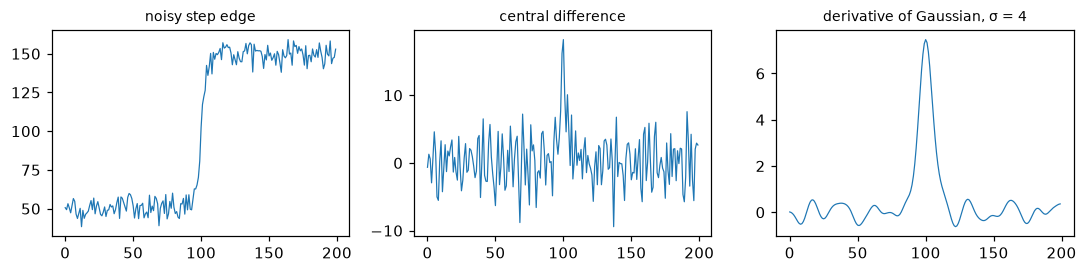
The central difference barely rises above its own noise. The derivative of Gaussian gives one clean peak at the edge, with a peak-to-noise ratio more than four times higher.

The gradient: magnitude and direction

An image is a function of two variables, so it has two partial derivatives. Together they form the gradient:

\[ \nabla f = \begin{pmatrix} g_x \\ g_y \end{pmatrix} = \begin{pmatrix} \partial f / \partial x \\ \partial f / \partial y \end{pmatrix}. \]

Here \(x\) is the column direction (rightward) and \(y\) is the row direction (downward in image coordinates, unlike the usual math convention). The gradient is a vector at every pixel, and as in calculus, it points in the direction of steepest increase of intensity. (The ML Handbook's Calculus and gradients derives this.) Two derived quantities matter:

• The gradient magnitude \(\lVert \nabla f \rVert = \sqrt{g_x^2 + g_y^2}\) is the edge strength: the rate of change in the steepest direction. Some implementations use \(\lvert g_x \rvert + \lvert g_y \rvert\), which is cheaper but not rotation-invariant.
• The gradient direction \(\theta = \operatorname{atan2}(g_y, g_x)\) points from dark to bright, perpendicular to the edge. The edge itself runs along \(\theta + 90°\). Use the two-argument atan2, which returns the full \((-180°, 180°]\) range, not arctan(gy / gx), which loses the sign and divides by zero on vertical edges.

Because the gradient direction is perpendicular to the edge, the gradient carries a lot of information beyond "there's an edge here": which side is brighter, and which way the edge runs. Histograms of gradient directions are the basis of the HOG and SIFT descriptors in Level 2.

Sobel, Prewitt, and Scharr

The classic derivative operators combine a central difference in one direction with a little smoothing in the other. The Sobel operator for \(g_x\) is

\[ S_x = \begin{pmatrix} -1 & 0 & 1 \\ -2 & 0 & 2 \\ -1 & 0 & 1 \end{pmatrix} = \begin{pmatrix} 1 \\ 2 \\ 1 \end{pmatrix} \begin{pmatrix} -1 & 0 & 1 \end{pmatrix}, \]

and \(S_y = S_x^\top\). It's separable: a central difference along \(x\) (unnormalized, so it's twice the slope) times a \([1, 2, 1]\) smoothing along \(y\), which is the 3-tap binomial approximation of a Gaussian. So Sobel is a tiny derivative-of-Gaussian. Its overall gain is 8: on a ramp with slope \(s\), the response is \(8s\). OpenCV leaves this factor in; scikit-image's sobel_h and sobel_v divide by 4.

The Prewitt operator uses \([1, 1, 1]\) smoothing instead. The Scharr operator uses \([3, 10, 3]\), with weights chosen to make the gradient direction as accurate as possible for all orientations. Sobel's direction estimate is off by up to a couple of degrees at some angles; Scharr's errors are several times smaller. Use Scharr when the direction matters (orientation histograms, optical flow); either is fine for edge strength. OpenCV's cv2.Sobel also supports larger apertures (5, 7) built from binomial smoothing and repeated differences.

from skimage import filters

img = data.camera()
f = img.astype(np.float64)
sobel_x = np.array([[-1, 0, 1], [-2, 0, 2], [-1, 0, 1]], float)
gx = ndimage.correlate(f, sobel_x, mode="mirror")              # mirror = OpenCV's default border
gy = ndimage.correlate(f, sobel_x.T, mode="mirror")
gx_cv = cv2.Sobel(img, cv2.CV_64F, 1, 0, ksize=3)                # float output: keep negatives!
gy_cv = cv2.Sobel(img, cv2.CV_64F, 0, 1, ksize=3)
print("matches cv2.Sobel:", np.allclose(gx, gx_cv), np.allclose(gy, gy_cv))
inner = (slice(1, -1), slice(1, -1))
print("skimage sobel_v = gx / 4:", np.allclose(filters.sobel_v(f)[inner], gx[inner] / 4))

# Direction accuracy: gradients of rotated sinusoids with known orientation
def worst_angle_error(kx):
    yy, xx = np.mgrid[:64, :64].astype(float)
    worst = 0.0
    for th in np.deg2rad(np.arange(0, 91, 5)):
        wave = np.sin(1.2 * (xx * np.cos(th) + yy * np.sin(th)))
        ax, ay = ndimage.correlate(wave, kx), ndimage.correlate(wave, kx.T)
        strong = np.hypot(ax, ay) > 0.5 * np.hypot(ax, ay).max()
        err = np.angle(np.exp(2j * (np.arctan2(ay, ax) - th))) / 2   # orientation error, mod 180
        worst = max(worst, np.rad2deg(np.median(np.abs(err[8:-8, 8:-8][strong[8:-8, 8:-8]]))))
    return worst

scharr_x = np.array([[-3, 0, 3], [-10, 0, 10], [-3, 0, 3]], float)
print(f"worst median direction error: Sobel {worst_angle_error(sobel_x):.2f} deg, "
      f"Scharr {worst_angle_error(scharr_x):.2f} deg")

matches cv2.Sobel: True True
skimage sobel_v = gx / 4: True
worst median direction error: Sobel 1.80 deg, Scharr 0.29 deg

Now let's look at the gradient of a real image. The direction is shown with color as hue (an angle), brightness proportional to magnitude, so you can see that opposite sides of a thin object have opposite gradient directions:

mag = np.hypot(gx, gy)
theta = np.arctan2(gy, gx)                                       # radians, (-pi, pi]
hsv = np.zeros(img.shape + (3,), np.uint8)
hsv[..., 0] = ((np.rad2deg(theta) % 360) / 2).astype(np.uint8)  # OpenCV hue: 0..179
hsv[..., 1] = 255
hsv[..., 2] = np.clip(mag / np.percentile(mag, 99) * 255, 0, 255).astype(np.uint8)
direction_rgb = cv2.cvtColor(hsv, cv2.COLOR_HSV2RGB)

fig, axes = plt.subplots(1, 4, figsize=(10, 2.7))
lim = np.percentile(np.abs(gx), 99)
for ax, (im, t, kw) in zip(axes, [(gx, "g_x (Sobel)", dict(cmap="RdBu_r", vmin=-lim, vmax=lim)),
                                  (gy, "g_y (Sobel)", dict(cmap="RdBu_r", vmin=-lim, vmax=lim)),
                                  (mag, "magnitude", dict(cmap="gray", vmax=np.percentile(mag, 99))),
                                  (direction_rgb, "direction (hue)", {})]):
    ax.imshow(im, **kw); ax.set_title(t, fontsize=9); ax.axis("off")
plt.tight_layout()
plt.show()

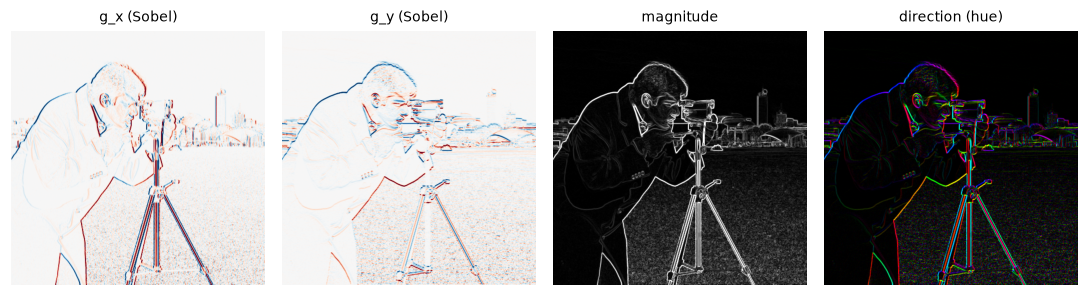
\(g_x\) responds to vertical edges and \(g_y\) to horizontal ones, with sign showing which side is brighter (red positive, blue negative). In the direction image, the two sides of each tripod leg have opposite colors.

Second derivatives: the Laplacian

At the center of a ramp edge, the first derivative has a maximum, so the second derivative crosses zero. Detecting edges as zero crossings of a second derivative is the other classic approach. In 2D, the rotation-invariant second derivative is the Laplacian:

\[ \nabla^2 f = \frac{\partial^2 f}{\partial x^2} + \frac{\partial^2 f}{\partial y^2}. \]

The 1D second difference is \(f(x+1) - 2f(x) + f(x-1)\), kernel \([1, -2, 1]\). Adding the \(x\) and \(y\) versions gives the 5-point Laplacian kernel \(\begin{smallmatrix} 0 & 1 & 0 \\ 1 & -4 & 1 \\ 0 & 1 & 0 \end{smallmatrix}\). It sums to zero (flat regions give zero), and it equals the difference between the average of the 4 neighbors and the pixel itself, times 4. A pixel brighter than its surroundings gives a negative Laplacian.

Its weaknesses: it's a second derivative, so it amplifies noise even more than the gradient does (it multiplies each frequency by its frequency squared). And it gives no direction, and it responds doubly to thin lines (zero crossings on both sides).

LoG and DoG

The fix is again to smooth first. The Laplacian of Gaussian (LoG) filters with \(\nabla^2 G_\sigma\):

\[ \nabla^2 G_\sigma(x, y) = \frac{x^2 + y^2 - 2\sigma^2}{\sigma^4}\, G_\sigma(x, y). \]

It's the "Mexican hat" (inverted): negative in a central disk of radius \(\sqrt{2}\sigma\), positive in a ring around it, summing to zero. The Marr-Hildreth edge detector (1980) takes the zero crossings of the LoG-filtered image. The LoG is also a blob detector: it responds most strongly to a dark or bright disk of radius about \(\sqrt{2}\sigma\), which is how scale-space blob detection and SIFT find keypoints in Level 2.

The LoG isn't separable, but a cheap approximation is: the difference of Gaussians (DoG), \(G_{k\sigma} - G_\sigma\). Here's why it works. The Gaussian satisfies the heat equation (a Gaussian is what heat diffusion produces from a point source):

\[ \frac{\partial G_\sigma}{\partial \sigma} = \sigma\, \nabla^2 G_\sigma. \]

You can check this by differentiating the formula. Now approximate the derivative with respect to \(\sigma\) by a finite difference:

\[ \frac{\partial G_\sigma}{\partial \sigma} \approx \frac{G_{k\sigma} - G_\sigma}{k\sigma - \sigma} \quad\Longrightarrow\quad G_{k\sigma} - G_\sigma \approx (k - 1)\,\sigma^2\, \nabla^2 G_\sigma. \]

The finite difference is most accurate at the middle of the interval, so the best-matching LoG has a scale between \(\sigma\) and \(k\sigma\) (the code below uses the geometric mean \(\sigma\sqrt{k}\)). So a DoG is a scaled LoG, and the scale factor \(\sigma^2\) is exactly the normalization that makes LoG responses comparable across scales. Marr and Hildreth suggested \(k \approx 1.6\); SIFT uses \(k = 2^{1/3} \approx 1.26\). Each Gaussian blur is separable and cheap, and in a pyramid you need the blurred images anyway, so DoGs come almost for free.

yy, xx = np.mgrid[-25:26, -25:26].astype(float)
def G(s):
    return np.exp(-(xx ** 2 + yy ** 2) / (2 * s * s)) / (2 * np.pi * s * s)
def LoG(s):
    return (xx ** 2 + yy ** 2 - 2 * s * s) / s ** 4 * G(s)

sigma = 3.0
for k in [1.6, 1.1]:
    dog_kernel = G(k * sigma) - G(sigma)
    s_mid = sigma * np.sqrt(k)                                  # the middle of [sigma, k*sigma] in log scale
    log_kernel = LoG(s_mid)
    corr = np.corrcoef(dog_kernel.ravel(), log_kernel.ravel())[0, 1]
    fit = (dog_kernel * log_kernel).sum() / (log_kernel ** 2).sum()
    print(f"k={k}: correlation {corr:.4f} | fitted scale {fit:.3f} | predicted (k-1)σ² {(k - 1) * s_mid ** 2:.3f}")

lap_raw = cv2.Laplacian(f, cv2.CV_64F, ksize=1)                 # the 5-point kernel
log_img = ndimage.gaussian_laplace(f, sigma=2.0)
dog_img = ndimage.gaussian_filter(f, 2.0 * 1.6) - ndimage.gaussian_filter(f, 2.0)

def zero_crossings(L, min_jump):
    """Pixels where L changes sign toward the right or down neighbor with a large enough jump."""
    zc = np.zeros(L.shape, bool)
    for a, b in [(L[:, :-1], L[:, 1:]), (L[:-1, :], L[1:, :])]:
        cross = (np.sign(a) != np.sign(b)) & (np.abs(a - b) > min_jump)
        zc[:a.shape[0], :a.shape[1]] |= cross
    return zc

zc = zero_crossings(log_img, min_jump=1.0)
fig, axes = plt.subplots(1, 4, figsize=(10, 2.7))
for ax, (im, t) in zip(axes, [(lap_raw, "Laplacian (no smoothing)"), (log_img, "LoG, σ = 2"),
                              (dog_img, "DoG, σ = 2 and 3.2"), (zc, "LoG zero crossings")]):
    lim = np.percentile(np.abs(im), 99) if im.dtype != bool else 1
    ax.imshow(im, cmap="gray", vmin=-lim if im.dtype != bool else 0, vmax=lim)
    ax.set_title(t, fontsize=9); ax.axis("off")
plt.tight_layout()
plt.show()

k=1.6: correlation 0.9986 | fitted scale 6.646 | predicted (k-1)σ² 8.640
k=1.1: correlation 1.0000 | fitted scale 0.943 | predicted (k-1)σ² 0.990

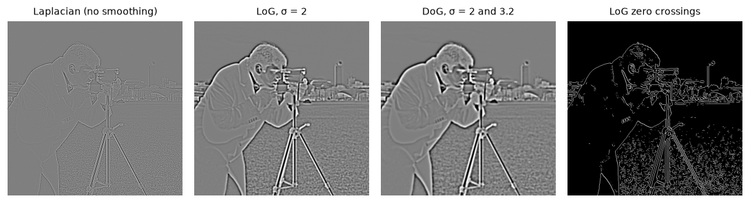
The raw Laplacian is dominated by fine texture. LoG and DoG look almost the same. Zero crossings of the LoG give closed contours, including some weak ones in the grass.

The DoG and LoG kernels have almost exactly the same shape (correlation above 0.998). The predicted scale factor is only roughly right for \(k = 1.6\), because a finite difference over such a wide interval is crude, and it gets close as \(k \to 1\). For finding zero crossings or extrema, a constant scale factor doesn't matter anyway. Zero crossings have a nice property, which you can see in the figure: they always form closed curves, because they're the boundary between positive and negative regions. But they also mark every gentle wiggle of intensity as an "edge", and they localize corners poorly. For most edge detection, Canny's gradient-based approach works better.

The Canny edge detector

In 1986 John Canny asked what an optimal edge detector would be, and stated three criteria:

1. Good detection: find real edges and few false ones (high signal-to-noise ratio).
2. Good localization: put each detected edge as close as possible to the true edge.
3. Single response: report each edge once, not as a thick band or several parallel lines.

For a step edge in white noise, his analysis showed that the optimal filter is well approximated by the derivative of a Gaussian, with a trade-off between criteria 1 and 2 controlled by \(\sigma\) (the uncertainty principle of edge detection). The rest of the algorithm enforces criterion 3 and makes the detection robust. The full pipeline:

flowchart LR
    A["Image"] --> B["1. Gaussian<br/>smoothing (σ)"]
    B --> C["2. Gradient<br/>(Sobel): magnitude<br/>and direction"]
    C --> D["3. Non-maximum<br/>suppression:<br/>thin to 1 pixel"]
    D --> E["4. Double threshold:<br/>strong, weak,<br/>discarded"]
    E --> F["5. Hysteresis:<br/>keep weak pixels<br/>connected to strong"]
    F --> G["Edge map"]

Step 1: smoothing. Blur with \(G_\sigma\) to suppress noise. This sets the scale of the edges you'll find.

Step 2: gradient. Compute \(g_x\) and \(g_y\) with Sobel, then the magnitude \(M = \sqrt{g_x^2 + g_y^2}\) and the direction \(\theta\). Steps 1 and 2 together are the derivative-of-Gaussian filter.

Step 3: non-maximum suppression (NMS). The magnitude around an edge is a ridge several pixels wide. The edge is the crest of the ridge, the point where the magnitude is a local maximum in the gradient direction (across the edge). For each pixel, look at its two neighbors along \(\pm\theta\) and keep the pixel only if its magnitude is at least as large as both. On a pixel grid, the direction is rounded to the nearest of four orientations: 0° (compare left and right), 45° (diagonal), 90° (compare up and down), and 135° (the other diagonal). Direction is taken modulo 180°, since \(\theta\) and \(\theta + 180°\) point along the same line. The result is ridges thinned to one pixel. (A more precise variant interpolates the magnitude at the exact positions along \(\theta\).)

Step 4: double threshold. Classify the surviving pixels with two thresholds, \(T_{\text{low}} < T_{\text{high}}\): strong if \(M > T_{\text{high}}\), weak if \(T_{\text{low}} < M \le T_{\text{high}}\), discarded otherwise.

Step 5: hysteresis. Keep every strong pixel. Keep a weak pixel only if it's connected (through a chain of weak or strong pixels, 8-connectivity) to a strong pixel. Weak pixels on their own are noise; weak pixels that continue a strong edge are part of it. The name comes from physics: like a thermostat that turns on at one temperature and off at another, an edge needs a strong signal to start but only a weak one to continue. This is what keeps faint stretches of Priya's cracks connected.

Building Canny from scratch

Here's every step in NumPy. For hysteresis, a neat trick replaces the usual stack-based tracing: label the connected components of the "weak or strong" mask with scipy.ndimage.label, then keep the components that contain at least one strong pixel.

def non_max_suppression(mag, theta_deg):
    """Keep pixels that are local maxima of mag along the (quantized) gradient direction."""
    q = (np.round((theta_deg % 180) / 45) % 4).astype(int)       # 0, 45, 90, 135 degrees
    steps = {0: (0, 1), 1: (1, 1), 2: (1, 0), 3: (1, -1)}          # (drow, dcol) along the gradient
    P = np.pad(mag, 1)
    H, W = mag.shape
    keep = np.zeros(mag.shape, bool)
    for d, (dr, dc) in steps.items():
        fwd = P[1 + dr:1 + dr + H, 1 + dc:1 + dc + W]
        bwd = P[1 - dr:1 - dr + H, 1 - dc:1 - dc + W]
        keep |= (q == d) & (mag > bwd) & (mag >= fwd)
    return np.where(keep, mag, 0.0)

def hysteresis(nms, low, high):
    candidates = nms > low
    labels, n = ndimage.label(candidates, structure=np.ones((3, 3)))   # 8-connectivity
    strong_ids = np.unique(labels[nms > high])
    return np.isin(labels, strong_ids[strong_ids > 0])

def canny(img_u8, low, high):
    """Canny on an already-smoothed uint8 image, with L2 magnitude (like OpenCV with L2gradient=True)."""
    f = img_u8.astype(np.float64)
    gx = cv2.Sobel(f, cv2.CV_64F, 1, 0, ksize=3)
    gy = cv2.Sobel(f, cv2.CV_64F, 0, 1, ksize=3)
    mag = np.hypot(gx, gy)
    nms = non_max_suppression(mag, np.rad2deg(np.arctan2(gy, gx)))
    return hysteresis(nms, low, high), mag, nms

smooth = cv2.GaussianBlur(img, (0, 0), 2.0)                       # step 1
low, high = 40, 100
edges, mag2, nms = canny(smooth, low, high)
edges_cv = cv2.Canny(smooth, low, high, L2gradient=True) > 0     # OpenCV does steps 2-5

both = np.count_nonzero(edges & edges_cv)
print("edge pixels: ours", edges.sum(), "| OpenCV", edges_cv.sum())
print("agreement (intersection over union):", round(both / np.count_nonzero(edges | edges_cv), 3))
near = ndimage.binary_dilation(edges_cv, np.ones((3, 3)))
print("our edge pixels within 1 px of an OpenCV edge:", round(np.mean(near[edges]), 4))

edge pixels: ours 5979 | OpenCV 5971
agreement (intersection over union): 0.999
our edge pixels within 1 px of an OpenCV edge: 1.0

The from-scratch detector reproduces OpenCV almost exactly: 99.9% of edge pixels match, and the rest are within one pixel. The small differences come from ties and from how each implementation quantizes directions near the 22.5° boundaries. Note that cv2.Canny does not smooth for you: it starts at step 2, with a 3 × 3 Sobel by default. scikit-image's feature.canny(img, sigma=...) includes the Gaussian step.

strong = nms > high
weak = (nms > low) & ~strong
crop = (slice(40, 296), slice(170, 426))
stages = [(smooth, "1. smoothed"), (mag2, "2. gradient magnitude"), (nms > 0, "3. after NMS"),
          (strong * 1.0 + weak * 0.4, "4. strong (white), weak (gray)"), (edges, "5. hysteresis (ours)"),
          (edges_cv, "cv2.Canny")]
fig, axes = plt.subplots(2, 3, figsize=(9, 6.2))
for ax, (im, t) in zip(axes.ravel(), stages):
    vmax = np.percentile(im, 99.5) if im.dtype == np.float64 and im.max() > 1 else None
    ax.imshow(im[crop], cmap="gray", vmax=vmax, interpolation="nearest")
    ax.set_title(t, fontsize=9); ax.axis("off")
plt.tight_layout()
plt.show()

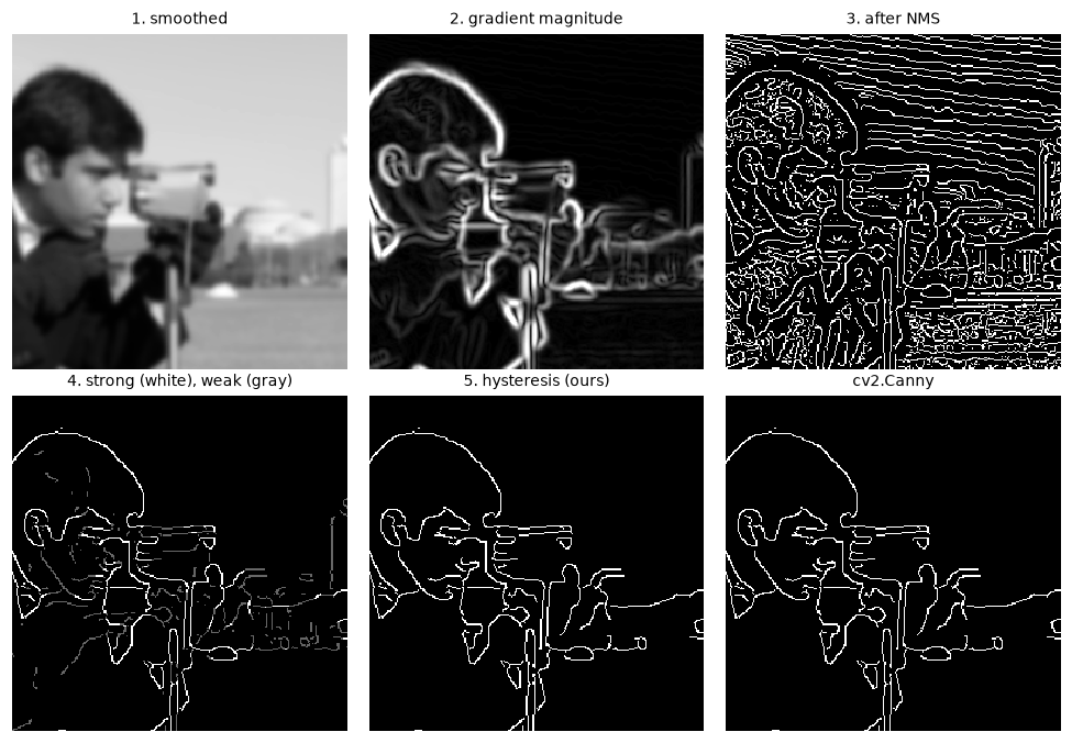
The thick magnitude ridges become one-pixel lines after NMS. Hysteresis keeps the weak pixels (gray) that continue strong edges and drops isolated ones. The last two panels are nearly identical.

Choosing σ and the thresholds

Canny has three parameters, and they interact:

• \(\sigma\) sets the scale. Start around 1 to 2 pixels for clean, detailed images, and go higher for noisy or textured ones.
• \(T_{\text{high}}\) decides which edges are worth starting. Raise it if you get too many spurious edges.
• \(T_{\text{low}}\) decides how far edges are followed. Canny recommended a ratio \(T_{\text{high}} : T_{\text{low}}\) of 2:1 to 3:1.

The thresholds are in units of gradient magnitude, which depends on the image's contrast and on the operator's gain (OpenCV's Sobel has gain 8, so on an 8-bit image magnitudes can reach about 1,440 with the L2 norm). Two common rules of thumb for picking them automatically, neither of them principled: set \(T_{\text{low}}\) and \(T_{\text{high}}\) to about 0.66 and 1.33 times the median of the image intensity (popular in tutorials, and it works surprisingly often on natural photos), or run Otsu on the gradient magnitudes and use its threshold as \(T_{\text{high}}\) and half of it as \(T_{\text{low}}\). scikit-image also accepts thresholds as quantiles of the magnitude (use_quantiles=True), which is the most robust to contrast changes.

In practice

The effect of σ

On a noisy image, \(\sigma\) decides whether you see edges or noise. Here's Canny on a synthetic scene of shapes with heavy noise, where the true edges are known, at three scales. To score each result, count the fraction of detected edge pixels within 2 pixels of a true edge (precision) and the fraction of true edge pixels within 2 pixels of a detection (recall):

from skimage import feature

rng = np.random.default_rng(1)
scene = np.full((200, 300), 90, np.uint8)
cv2.rectangle(scene, (30, 40), (120, 160), 160, -1)
cv2.circle(scene, (210, 100), 55, 130, -1)
cv2.line(scene, (140, 20), (280, 190), 60, 3)
truth = cv2.Canny(scene, 10, 20) > 0                            # edges of the clean scene
noisy_scene = np.clip(scene + rng.normal(0, 25, scene.shape), 0, 255).astype(np.uint8)

def score(det, truth, tol=2):
    near_truth = ndimage.binary_dilation(truth, iterations=tol)
    near_det = ndimage.binary_dilation(det, iterations=tol)
    return near_truth[det].mean(), near_det[truth].mean()

fig, axes = plt.subplots(1, 4, figsize=(10, 2.2))
axes[0].imshow(noisy_scene, cmap="gray"); axes[0].set_title("noisy scene (σ_noise = 25)", fontsize=9)
for ax, s in zip(axes[1:], [1.0, 2.5, 5.0]):
    det = feature.canny(noisy_scene, sigma=s, low_threshold=0.7, high_threshold=0.9, use_quantiles=True)
    p, r = score(det, truth)
    ax.imshow(det, cmap="gray"); ax.set_title(f"σ = {s}: precision {p:.2f}, recall {r:.2f}", fontsize=8)
    print(f"sigma={s}: precision {p:.2f}  recall {r:.2f}")
for ax in axes:
    ax.axis("off")
plt.tight_layout()
plt.show()

sigma=1.0: precision 0.18  recall 1.00
sigma=2.5: precision 0.98  recall 0.99
sigma=5.0: precision 0.75  recall 0.56

At σ = 1 the noise produces edge fragments everywhere. At σ = 2.5 the shapes come out cleanly. At σ = 5 the noise is gone, but the corners round off and the thin dark line disappears outside the circle: its two edges are only 3 pixels apart, and heavy blurring flattens it.

The middle scale is nearly perfect. At the smallest scale, recall is perfect but most detections are noise. At the largest scale, both numbers drop: blurring merges the line's two edges and rounds the corners, so many detections drift more than 2 pixels from the true edges, and parts of the true edges are no longer found. This is Canny's detection-versus-localization trade-off in numbers.

Estimating document skew from gradient directions

Gradient directions are useful on their own. Text has strong horizontal structure (baselines, the tops and bottoms of letters) and vertical strokes. Rotate a page, and the peaks of the magnitude-weighted histogram of gradient orientations rotate with it. That gives a fast skew estimate for document images:

from skimage import transform

text = data.text()
true_angle = 7.0
rotated = transform.rotate(text, true_angle, resize=True, mode="edge", preserve_range=True)
gx_r = cv2.Sobel(rotated, cv2.CV_64F, 1, 0, ksize=3)
gy_r = cv2.Sobel(rotated, cv2.CV_64F, 0, 1, ksize=3)
orient = np.rad2deg(np.arctan2(gy_r, gx_r)) % 180                # orientation, not direction
hist, edges_deg = np.histogram(orient, bins=180, range=(0, 180), weights=np.hypot(gx_r, gy_r))
peak = edges_deg[np.argmax(hist)] + 0.5
# Horizontal text lines have vertical gradients (90 deg); their tilt shows up as the peak's offset
skew = (peak - 90 + 45) % 90 - 45
print(f"histogram peak at {peak:.1f} deg -> estimated skew {abs(skew):.1f} deg (true {true_angle})")

histogram peak at 173.5 deg -> estimated skew 6.5 deg (true 7.0)

The rotated page's strongest orientation gives its tilt to within a degree (the histogram has 1° bins), folded into \(\pm 45°\) because horizontal and vertical structures both count. Deskewing by that angle (with the rotation in Geometric transformations) is a standard step before OCR. A more robust variant uses the Hough transform on the edge map, or projection profiles: rotate by candidate angles and pick the one whose row sums are most peaked.

Common mistake: Sobel into uint8

cv2.Sobel(img, -1, 1, 0) on a uint8 image keeps uint8, so negative derivatives (bright-to-dark transitions) are clipped to 0 and the magnitude is wrong. Use cv2.CV_64F (or CV_32F, or CV_16S followed by cv2.convertScaleAbs for display only).

Common mistake: forgetting that y points down

In image coordinates, \(y\) (the row index) increases downward. A gradient of \(\theta = 90°\) points down the image (bright below), not up. Mixing this with a math-convention plot, or with (x, y) vs (row, col) order in NumPy indexing, flips directions. Keep gx for columns and gy for rows, and use np.arctan2(gy, gx).

Common mistake: running cv2.Canny on an unsmoothed noisy image

cv2.Canny uses only a 3 × 3 Sobel, which is very little smoothing. On noisy images, blur first with cv2.GaussianBlur, or use skimage.feature.canny, which takes sigma.

Exercises

Exercise 1: Sobel by hand (easy)

Compute the Sobel \(g_x\), \(g_y\), magnitude, and direction at the center of each 3 × 3 patch by hand, then check with code:

\[ A = \begin{pmatrix} 10 & 10 & 50 \\ 10 & 10 & 50 \\ 10 & 10 & 50 \end{pmatrix}, \qquad B = \begin{pmatrix} 10 & 10 & 10 \\ 10 & 10 & 50 \\ 10 & 50 & 50 \end{pmatrix}. \]

Solution

For \(A\): \(g_x = (50 - 10)(1 + 2 + 1) = 160\), \(g_y = 0\). Magnitude 160, direction 0°: the gradient points right, toward the bright column, perpendicular to the vertical edge.

For \(B\): \(g_x = (-1)(10) + (1)(10) + (-2)(10) + (2)(50) + (-1)(10) + (1)(50) = 120\). By symmetry \(g_y = 120\). Magnitude \(120\sqrt{2} \approx 169.7\), direction 45°: down and to the right, toward the bright corner (remember \(y\) points down).

for name, P in [("A", [[10, 10, 50]] * 3), ("B", [[10, 10, 10], [10, 10, 50], [10, 50, 50]])]:
    P = np.array(P, float)
    px, py = (sobel_x * P).sum(), (sobel_x.T * P).sum()
    print(name, "gx", px, "gy", py, "mag", round(np.hypot(px, py), 1), "dir", np.rad2deg(np.arctan2(py, px)))

A gx 160.0 gy 0.0 mag 160.0 dir 0.0
B gx 120.0 gy 120.0 mag 169.7 dir 45.0

Exercise 2: The LoG on simple signals (easy)

Before running anything, predict the response of a LoG filter on (a) a constant image, (b) a linear ramp \(f = 3x + 2y\), and (c) a single bright pixel. Explain each prediction from the formula, then check with ndimage.gaussian_laplace (look at interior pixels).

Solution

(a) Zero: the LoG kernel sums to zero. (b) Zero: the Laplacian of a linear function is zero (second derivatives vanish), and smoothing a ramp gives the same ramp. Unlike the gradient, the Laplacian ignores constant slopes. (c) The kernel itself, centered at the pixel: a negative center (since \(\nabla^2 G < 0\) inside radius \(\sqrt{2}\sigma\)) surrounded by a positive ring.

yy, xx = np.mgrid[:64, :64].astype(float)
flat, ramp = np.full((64, 64), 7.0), 3 * xx + 2 * yy
dot = np.zeros((64, 64)); dot[32, 32] = 100
inner = (slice(16, -16), slice(16, -16))
print("flat: max |LoG|", np.abs(ndimage.gaussian_laplace(flat, 2))[inner].max().round(8))
print("ramp: max |LoG|", np.abs(ndimage.gaussian_laplace(ramp, 2))[inner].max().round(8))
resp = ndimage.gaussian_laplace(dot, 2)
print("dot: center", resp[32, 32].round(3), "| at distance 4:", resp[32, 36].round(3))

flat: max |LoG| 0.00121362
ramp: max |LoG| 0.04074297
dot: center -1.99 | at distance 4: 0.269

The flat and ramp responses are tiny but not exactly zero: SciPy samples and truncates the kernel, so its weights don't sum to exactly zero, and on a ramp with values in the hundreds that leaves a residue of a few hundredths. Compared with the dot's response, that's negligible. At distance 4 (beyond \(\sqrt{2}\sigma \approx 2.8\)) the dot's response is positive, in the ring.

Exercise 3: Why hysteresis? (medium)

On noisy_scene from this chapter, smoothed with \(\sigma = 1.5\), compare three edge maps: a single threshold at \(T_{\text{low}}\), a single threshold at \(T_{\text{high}}\) (both after NMS), and hysteresis with both. For each, report precision, recall, and the number of connected edge fragments. Use the 75th and 95th percentiles of the NMS-surviving magnitudes as the thresholds.

Solution

sm = cv2.GaussianBlur(noisy_scene, (0, 0), 1.5)
fx = cv2.Sobel(sm.astype(float), cv2.CV_64F, 1, 0); fy = cv2.Sobel(sm.astype(float), cv2.CV_64F, 0, 1)
nm = non_max_suppression(np.hypot(fx, fy), np.rad2deg(np.arctan2(fy, fx)))
lo, hi = np.percentile(nm[nm > 0], [75, 95])
for name, det in [("low only", nm > lo), ("high only", nm > hi), ("hysteresis", hysteresis(nm, lo, hi))]:
    p, r = score(det, truth)
    n = ndimage.label(det, structure=np.ones((3, 3)))[1]
    print(f"{name:11s} precision {p:.2f}  recall {r:.2f}  fragments {n}")

low only    precision 0.30  recall 1.00  fragments 824
high only   precision 1.00  recall 0.74  fragments 31
hysteresis  precision 0.97  recall 0.98  fragments 10

The low threshold alone finds all the true edges but buries them in hundreds of noise fragments. The high threshold alone is clean but broken: a quarter of the true edges are missing, and the rest come in about 30 pieces. Hysteresis gets nearly the recall of the low threshold and nearly the precision of the high one, with the fewest fragments of all three, because it only keeps weak pixels that continue strong edges. That's exactly the "start strong, continue weak" behavior that kept Priya's cracks connected.

Exercise 4: Sub-pixel edge location (hard)

Edges don't fall on pixel centers. Create a 1D blurred step whose true edge is at \(x = 40.3\): 0.5 * (1 + erf((x - 40.3) / (np.sqrt(2) * 1.5))) scaled to 0–200. Find the integer peak of the central-difference gradient, then refine it by fitting a parabola through the peak and its two neighbors. Derive the parabola's vertex formula and report your estimate's error.

Solution

Fit \(y = a t^2 + b t + c\) through \((-1, y_{-1})\), \((0, y_0)\), \((1, y_1)\). Then \(c = y_0\), \(b = \frac{y_1 - y_{-1}}{2}\), and \(a = \frac{y_1 - 2y_0 + y_{-1}}{2}\). The vertex is at \(t^* = -\frac{b}{2a} = \frac{y_{-1} - y_1}{2(y_{-1} - 2y_0 + y_1)}\), an offset in \((-\frac12, \frac12)\) from the integer peak.

from scipy.special import erf

xs1 = np.arange(80, dtype=float)
sig = 200 * 0.5 * (1 + erf((xs1 - 40.3) / (np.sqrt(2) * 1.5)))
grad = np.convolve(sig, [0.5, 0, -0.5], mode="same")       # central difference
i = int(np.argmax(grad[1:-1])) + 1
ym, y0, yp = grad[i - 1], grad[i], grad[i + 1]
offset = (ym - yp) / (2 * (ym - 2 * y0 + yp))
print("integer peak:", i, "| refined:", round(i + offset, 3), "| error:", round(abs(i + offset - 40.3), 3))

integer peak: 40 | refined: 40.282 | error: 0.018

The integer peak is off by 0.3 pixels; the parabola fit cuts the error to about two hundredths of a pixel on this clean signal (the remaining bias comes from the gradient peak not being exactly a parabola). With noise, the accuracy is typically around a tenth of a pixel. Sub-pixel edge localization like this is what makes optical gauging (measuring parts from images) and camera calibration precise. In 2D, apply the same fit along the gradient direction at each NMS pixel.

Exercise 5: Edges that grayscale can't see (hard)

Make an image whose left half is pure red (200, 60, 60) and right half a green with the same grayscale value under cv2.COLOR_RGB2GRAY. Show that Canny on the grayscale image finds no edge. Then compute a color gradient: Sobel on each channel, and at each pixel take the channel with the largest magnitude. Show that the color edge is found.

Solution

Grayscale is \(Y = 0.299R + 0.587G + 0.114B\). For the red, \(Y = 0.299 \cdot 200 + 0.587 \cdot 60 + 0.114 \cdot 60 = 101.9\). A green with \(R = 60\) and \(B = 60\) needs \(0.587G = 101.9 - 24.78\), so \(G \approx 131\).

iso = np.zeros((100, 160, 3), np.uint8)
iso[:, :80] = (200, 60, 60)
iso[:, 80:] = (60, 131, 60)
gray = cv2.cvtColor(iso, cv2.COLOR_RGB2GRAY)
print("gray values:", np.unique(gray), "| Canny edge pixels on gray:", np.count_nonzero(cv2.Canny(gray, 20, 40)))

mags = [np.hypot(cv2.Sobel(iso[..., c].astype(float), cv2.CV_64F, 1, 0),
                 cv2.Sobel(iso[..., c].astype(float), cv2.CV_64F, 0, 1)) for c in range(3)]
color_mag = np.max(mags, axis=0)
cols = np.flatnonzero(color_mag.max(axis=0) > 100)
print("columns with a strong color gradient:", cols)

gray values: [102] | Canny edge pixels on gray: 0
columns with a strong color gradient: [79 80]

The two colors are isoluminant: different hues, identical brightness. Any detector on the grayscale image is blind to the boundary, while the per-channel gradient sees a jump of 140 in red and 71 in green. cv2.Canny on a 3-channel image does this max-over-channels internally. A more principled color gradient uses the structure tensor (Di Zenzo's method), summing the outer products of all channels' gradients and taking the largest eigenvalue, an idea you'll meet again in the Harris corner detector.

Check yourself

1. Why is the central difference preferred over the forward difference for image derivatives?

   Answer

   Its error is \(O(h^2)\) instead of \(O(h)\), because the even Taylor terms cancel, and it's centered on the pixel, so it doesn't shift edges by half a pixel.

2. Why must you smooth before differentiating, and what's the trade-off in choosing \(\sigma\)?

   Answer

   Differentiation amplifies high-frequency noise relative to the edge signal. Smoothing with a Gaussian restores the signal-to-noise ratio. Larger \(\sigma\) suppresses more noise and finds coarser edges but localizes them worse and merges nearby edges.

3. What do the gradient magnitude and direction tell you, and how is the direction related to the edge?

   Answer

   The magnitude is the edge strength; the direction points from dark to bright, perpendicular to the edge. The edge runs at \(\theta + 90°\).

4. Why is Sobel separable, and what are its two 1D factors?

   Answer

   It's an outer product: \([1, 2, 1]^\top\) smoothing across the derivative direction times \([-1, 0, 1]\) central difference along it.

5. Why does a DoG approximate a LoG?

   Answer

   The Gaussian satisfies the heat equation \(\partial G / \partial \sigma = \sigma \nabla^2 G\). Approximating the \(\sigma\)-derivative by a finite difference gives \(G_{k\sigma} - G_\sigma \approx (k - 1)\sigma^2 \nabla^2 G_\sigma\).

6. What does non-maximum suppression do, and why does it need the gradient direction?

   Answer

   It thins the magnitude ridges to one pixel by keeping only pixels that are local maxima across the edge. Across the edge means along the gradient direction, so the direction tells NMS which two neighbors to compare against.

7. What problem does hysteresis solve that a single threshold can't?

   Answer

   A single threshold forces a choice between noise (too low) and broken edges (too high). Hysteresis uses the high threshold to start edges and the low one to continue them, so faint stretches of real edges survive while isolated weak responses are dropped.

8. Does cv2.Canny smooth the image for you?

   Answer

   No. It computes a 3 × 3 (or larger aperture) Sobel directly. Blur with cv2.GaussianBlur first, or use skimage.feature.canny, which takes a sigma.

Key takeaways

• Edges are rapid intensity changes; first derivatives peak and second derivatives cross zero at them.
• Central differences are accurate to \(O(h^2)\), but any derivative amplifies noise, so smooth first. Smoothing then differentiating equals one derivative-of-Gaussian filter.
• The gradient \((g_x, g_y)\) gives edge strength and a direction perpendicular to the edge. Sobel is a separable mini derivative-of-Gaussian; Scharr gets directions more accurately.
• The Laplacian is a rotation-invariant second derivative; LoG smooths it, DoG approximates LoG cheaply via the heat equation, and both double as blob detectors.
• Canny = Gaussian smoothing + gradient + non-maximum suppression + double threshold + hysteresis. Each step fixes a specific failure of naive edge detection.
• Keep derivatives in float, remember that \(y\) points down, and pick \(\sigma\) for the scale of the edges you want.

Further reading

• John Canny, "A Computational Approach to Edge Detection", IEEE Transactions on Pattern Analysis and Machine Intelligence, 1986. The original derivation of the criteria and the detector.
• David Marr and Ellen Hildreth, "Theory of Edge Detection", Proceedings of the Royal Society of London B, 1980. LoG and zero crossings.
• Richard Szeliski, Computer Vision: Algorithms and Applications, 2nd edition, section 7.2 (edges and contours), free at szeliski.org/Book.
• OpenCV tutorials: Image gradients and Canny edge detection.

Next

Smoothing, sharpening, and differentiating all have a cleaner description as operations on frequencies. Next: The frequency domain.