Stereo and multi-view geometry
Level 2 · Chapter 4 · ⏱️ ~85 min read · Prerequisites: Cameras and calibration, Matching and RANSAC
One image loses depth; two images taken from different positions bring it back. This chapter develops the geometry of two views: epipolar lines, the essential and fundamental matrices, the normalized eight-point algorithm (which you'll implement), recovering the relative camera pose, and triangulating 3D points. Then it turns to dense stereo: rectification, the relationship between disparity and depth, block matching, and semi-global matching (also implemented from scratch), evaluated against ground-truth disparity on a real Middlebury stereo pair. It closes with an overview of structure from motion, which scales the same ideas to thousands of images.
Why it matters
Priya's team was building a small warehouse robot that needed to see pallets and people in front of it. They chose a cheap stereo camera module over a lidar to save cost, ran OpenCV's block matcher out of the box, and got depth maps that looked plausible in the demo room.
In the warehouse, the depth maps had holes on the plain gray floor and on the white shrink-wrapped pallets, and objects beyond about 6 meters jittered by a meter from frame to frame. Both problems are predictable from first principles. Block matching needs texture to match, and plain surfaces don't have any. And depth from stereo is \(Z = fB/d\), so a fixed half-pixel uncertainty in disparity becomes a depth uncertainty that grows with \(Z^2\): with their 6 cm baseline, half a pixel at 6 meters was worth almost a meter.
Knowing the geometry, the fixes were clear: a wider baseline (12 cm halved the far-range error), semi-global matching instead of plain block matching (smoother surfaces, fewer holes), a projected infrared texture pattern for blank surfaces (the trick used by many active stereo cameras), and a hard limit on trusted range. This chapter gives you the formulas and the algorithms behind each of those decisions.
Concepts
Two views of one point
Two cameras with centers \(\mathbf{C}_1\) and \(\mathbf{C}_2\) look at a 3D point \(\mathbf{X}\). It appears at \(\mathbf{x}_1\) in image 1 and \(\mathbf{x}_2\) in image 2. The line between the two camera centers is the baseline.
Suppose you know \(\mathbf{x}_1\) and want to find \(\mathbf{x}_2\). You don't know the depth of \(\mathbf{X}\), so it could be anywhere on the ray from \(\mathbf{C}_1\) through \(\mathbf{x}_1\). Project that whole ray into image 2: it becomes a line. So the match for \(\mathbf{x}_1\) must lie on a known line in image 2, the epipolar line of \(\mathbf{x}_1\). The search for a correspondence drops from 2D to 1D. That's the single most important fact in multi-view geometry.
The vocabulary:
- The epipolar plane is the plane through \(\mathbf{C}_1\), \(\mathbf{C}_2\), and \(\mathbf{X}\). Every 3D point defines one, and they all contain the baseline (a "book" of planes hinged on the baseline).
- An epipolar line is the intersection of an epipolar plane with an image plane.
- The epipole \(\mathbf{e}_2\) is where the baseline pierces image plane 2, which is the image of camera center \(\mathbf{C}_1\) in camera 2 (and vice versa for \(\mathbf{e}_1\)). All epipolar lines in an image pass through its epipole. When the cameras are side by side with parallel optical axes, the epipoles are at infinity and the epipolar lines are parallel and horizontal: that's the rectified stereo case.
The essential matrix
Work in normalized coordinates (from the previous chapter), \(\hat{\mathbf{x}} = \mathbf{K}^{-1}\tilde{\mathbf{u}}\), so the intrinsics are out of the way. Put camera 1 at the origin with no rotation. Camera 2 is related by \(\mathbf{X}_2 = \mathbf{R}\mathbf{X}_1 + \mathbf{t}\): a point with coordinates \(\mathbf{X}_1\) in camera 1's frame has coordinates \(\mathbf{X}_2\) in camera 2's frame.
The point \(\mathbf{X}_1\) lies along \(\hat{\mathbf{x}}_1\) (it's \(Z_1\hat{\mathbf{x}}_1\)), and \(\mathbf{X}_2 = Z_2\hat{\mathbf{x}}_2\). Express all three vectors of the epipolar plane in camera 2's frame:
- the ray to the point, \(\hat{\mathbf{x}}_2\) (up to scale);
- the baseline, which is the vector from camera 2's center to camera 1's center, \(\mathbf{t}\);
- the ray from camera 1 to the point, rotated into camera 2's frame, \(\mathbf{R}\hat{\mathbf{x}}_1\).
These three vectors lie in one plane (the epipolar plane), so they're coplanar, and their scalar triple product is zero:
Write the cross product as a matrix product with the cross-product matrix \([\mathbf{t}]_\times\) (the same construction as in Rodrigues' formula):
\(\mathbf{E}\) is the essential matrix (Longuet-Higgins, 1981). It encodes the relative pose of the two cameras in a single \(3 \times 3\) matrix. Its properties follow from its form:
- Rank 2. \([\mathbf{t}]_\times\) has rank 2 (it maps \(\mathbf{t}\) to zero), so \(\mathbf{E}\) does too.
- Two equal singular values. The singular values of \(\mathbf{E}\) are \((\sigma, \sigma, 0)\) with \(\sigma = \lVert\mathbf{t}\rVert\), because \(\mathbf{R}\) is orthogonal and \([\mathbf{t}]_\times\) has singular values \((\lVert\mathbf{t}\rVert, \lVert\mathbf{t}\rVert, 0)\).
- Five degrees of freedom. Three for rotation, three for translation, minus one because the constraint \(= 0\) is unchanged if you scale \(\mathbf{E}\), so the scale of the translation can't be recovered from images alone. A scene twice as large, seen from cameras twice as far apart, looks identical. You need a known distance (a baseline measurement, an object of known size) to fix the scale.
The fundamental matrix
In pixel coordinates, substitute \(\hat{\mathbf{x}}_i = \mathbf{K}_i^{-1}\tilde{\mathbf{u}}_i\):
\(\mathbf{F}\) is the fundamental matrix. It's the uncalibrated version of \(\mathbf{E}\): you can estimate it from pixel correspondences alone, without knowing either camera's intrinsics. It has rank 2 (like \(\mathbf{E}\)) and 7 degrees of freedom (9 entries, minus scale, minus the rank-2 constraint \(\det\mathbf{F} = 0\)).
The geometry falls out of matrix-vector products:
- The epipolar line in image 2 of a point \(\tilde{\mathbf{u}}_1\) is \(\mathbf{l}_2 = \mathbf{F}\tilde{\mathbf{u}}_1\), a line \((a, b, c)\) meaning \(au + bv + c = 0\). The constraint \(\tilde{\mathbf{u}}_2^\top\mathbf{l}_2 = 0\) says exactly that \(\tilde{\mathbf{u}}_2\) lies on it. Similarly \(\mathbf{l}_1 = \mathbf{F}^\top\tilde{\mathbf{u}}_2\).
- The epipoles are the null vectors: \(\mathbf{F}\mathbf{e}_1 = \mathbf{0}\) and \(\mathbf{F}^\top\mathbf{e}_2 = \mathbf{0}\). Every epipolar line passes through the epipole, so \(\mathbf{l}_2^\top\mathbf{e}_2 = \tilde{\mathbf{u}}_1^\top\mathbf{F}^\top\mathbf{e}_2 = 0\) for all \(\tilde{\mathbf{u}}_1\). This is why rank 2 is essential: a full-rank \(\mathbf{F}\) would have no epipoles, and its epipolar lines wouldn't meet at a point.
- The distance of \(\tilde{\mathbf{u}}_2\) from its epipolar line, \(|\tilde{\mathbf{u}}_2^\top\mathbf{F}\tilde{\mathbf{u}}_1| / \sqrt{l_a^2 + l_b^2}\), is a pixel-level measure of how well a match fits \(\mathbf{F}\). The Sampson distance, a first-order approximation of the geometric reprojection error, is what RANSAC uses as the residual:
The eight-point algorithm
How do you estimate \(\mathbf{F}\) from matches? The constraint \(\tilde{\mathbf{u}}_2^\top\mathbf{F}\tilde{\mathbf{u}}_1 = 0\) is linear in the entries of \(\mathbf{F}\). With \(\tilde{\mathbf{u}}_1 = (x, y, 1)\), \(\tilde{\mathbf{u}}_2 = (x', y', 1)\), and \(\mathbf{f}\) the 9 entries of \(\mathbf{F}\) in row-major order, it expands to
Each correspondence gives one equation (not two, as for a homography: a point constrains its match only to a line, not to a point). Stack \(n \ge 8\) of them into \(\mathbf{A}\mathbf{f} = \mathbf{0}\), and solve by SVD, exactly like the DLT. That's the eight-point algorithm (Longuet-Higgins 1981, made practical by Hartley 1997). Two steps are essential:
- Normalize. As with the DLT, transform each image's points so their centroid is at the origin and their mean distance is \(\sqrt{2}\). Hartley's paper was titled "In Defense of the Eight-Point Algorithm" because, without normalization, the algorithm was considered hopelessly unstable; with it, it's competitive with iterative methods.
- Enforce rank 2. The least-squares solution of \(\mathbf{A}\mathbf{f} = \mathbf{0}\) won't have \(\det\mathbf{F} = 0\) exactly. Replace it with the closest rank-2 matrix (in Frobenius norm): take its SVD \(\mathbf{U}\operatorname{diag}(\sigma_1, \sigma_2, \sigma_3)\mathbf{V}^\top\) and set \(\sigma_3 = 0\).
Then denormalize: \(\mathbf{F} = \mathbf{T}_2^\top\,\tilde{\mathbf{F}}\,\mathbf{T}_1\) (the transpose appears because \(\mathbf{F}\) is sandwiched between the two points).
With outliers, wrap it in RANSAC. The minimal seven-point algorithm uses the rank-2 constraint directly (giving a cubic with one or three real solutions) and needs far fewer RANSAC iterations than eight points: at 50% inliers, 588 versus 1,177 for 99% confidence. For calibrated cameras, the five-point algorithm (Nistér, 2004) estimates \(\mathbf{E}\) directly from five matches; cv2.findEssentialMat uses it inside RANSAC.
Degenerate scenes
If all the 3D points lie on a single plane, or the camera only rotates without translating, \(\mathbf{F}\) is not determined by the matches: there's a whole family of fundamental matrices consistent with them (the matches are explained by a homography instead). Robust pipelines test both models (homography and fundamental matrix) and choose by a model-selection criterion, as ORB-SLAM does during initialization.
Recovering the pose from E
If you know the intrinsics, \(\mathbf{E} = \mathbf{K}_2^\top\mathbf{F}\mathbf{K}_1\), and you can extract \(\mathbf{R}\) and \(\mathbf{t}\). Take the SVD \(\mathbf{E} = \mathbf{U}\operatorname{diag}(1, 1, 0)\mathbf{V}^\top\) (making sure \(\mathbf{U}\) and \(\mathbf{V}\) are rotations, with determinant \(+1\)), and let
Then \(\mathbf{R} \in \{\mathbf{U}\mathbf{W}\mathbf{V}^\top,\; \mathbf{U}\mathbf{W}^\top\mathbf{V}^\top\}\) and \(\mathbf{t} = \pm\mathbf{u}_3\) (the last column of \(\mathbf{U}\), unit length). That's four candidate poses. Only one puts the triangulated points in front of both cameras (positive depth in both); this test is called the cheirality check. You'll implement it below and compare with cv2.recoverPose, which does the same.
Triangulation
With both projection matrices \(\mathbf{P}_1 = \mathbf{K}_1[\mathbf{I} \mid \mathbf{0}]\) and \(\mathbf{P}_2 = \mathbf{K}_2[\mathbf{R} \mid \mathbf{t}]\), each match gives two rays, and the 3D point is where they meet. With noise, the rays don't quite intersect. The linear (DLT) triangulation writes, for each camera, \(\tilde{\mathbf{u}} \times (\mathbf{P}\tilde{\mathbf{X}}) = \mathbf{0}\), which gives two independent equations per view. With rows \(\mathbf{p}^{1\top}, \mathbf{p}^{2\top}, \mathbf{p}^{3\top}\) of \(\mathbf{P}\) and pixel \((u, v)\):
Four equations, four homogeneous unknowns (three after scale): solve by SVD again. cv2.triangulatePoints implements this. The result minimizes an algebraic error; the optimal triangulation (Hartley and Sturm, 1997) minimizes reprojection error and matters when rays are nearly parallel.
Triangulation accuracy depends on the angle between the rays. Points far away relative to the baseline have nearly parallel rays, and a small pixel error moves the intersection a long way along the rays. That's the same \(Z^2\) effect you'll see in stereo depth below.
Rectification
Searching along arbitrary epipolar lines is awkward. Stereo rectification warps both images (by a homography each, after undistortion) so that the epipolar lines become horizontal and aligned: a point in row \(v\) of the left image has its match in row \(v\) of the right image. Geometrically, rectification rotates both cameras virtually so that their image planes are coplanar and parallel to the baseline, and gives them the same intrinsics.
cv2.stereoRectify(K1, d1, K2, d2, size, R, T) computes the two rectifying rotations \(\mathbf{R}_1, \mathbf{R}_2\), new projection matrices \(\mathbf{P}_1, \mathbf{P}_2\), and a \(4 \times 4\) reprojection matrix \(\mathbf{Q}\) that maps (pixel, disparity) to 3D. cv2.initUndistortRectifyMap and cv2.remap then produce the rectified images. For uncalibrated pairs, cv2.stereoRectifyUncalibrated computes rectifying homographies from \(\mathbf{F}\) alone.
Disparity and depth
In a rectified pair with focal length \(f\) (pixels) and baseline \(B\), a point at depth \(Z\) appears at column \(x_L\) in the left image and \(x_R\) in the right. The disparity is \(d = x_L - x_R\). By similar triangles, with the left camera at the origin and the right camera at \((B, 0, 0)\):
If the two rectified cameras have different principal points (as in the Middlebury data used below), there's a constant offset: \(Z = fB/(d + d_{\text{offs}})\) with \(d_{\text{offs}} = c_{x,R} - c_{x,L}\).
Depth is inversely proportional to disparity. Near objects have large disparities; distant ones have small disparities, and infinitely far points have zero. Differentiate to see how disparity errors become depth errors:
Depth error grows with the square of the distance, and shrinks with a longer baseline or a longer focal length. This is the formula behind Priya's robot: with \(f = 700\) px, \(B = 0.06\) m, and \(\Delta d = 0.5\) px, the error at 6 m is \(36/(42) \times 0.5 \approx 0.43\) m, and at 10 m it's 1.2 m. The trade-off is that a longer baseline makes matching harder (the views differ more, more points are occluded in one view) and increases the minimum depth that fits in the disparity search range.
Block matching
Dense stereo computes a disparity for every pixel of the (rectified) left image. The simplest method is block matching: for each pixel, compare a small window around it with windows at each candidate disparity \(d \in [d_{\min}, d_{\max})\) along the same row of the right image, and pick the best. Common costs:
- SAD (sum of absolute differences) or SSD (sum of squared differences): fast, but sensitive to brightness differences between the cameras.
- NCC (normalized cross-correlation): subtracts the window means and divides by the standard deviations, so it's invariant to gain and offset.
- Census transform: encode each pixel by a bit string of comparisons with its neighbors (like BRIEF), then compare bit strings with the Hamming distance. Robust to any monotonic brightness change, and the standard data cost in many practical systems.
Computing all costs for all pixels and disparities gives a cost volume \(C(x, y, d)\). Choosing \(\arg\min_d C(x, y, d)\) at each pixel independently is called winner-take-all. The window size is the central trade-off: small windows are noisy (too little texture to be distinctive) but preserve edges; large windows are smoother but blur depth discontinuities ("foreground fattening": the window straddles a near object and its background, and the strong texture of the object wins).
Post-processing turns raw winners into trustworthy estimates:
- Sub-pixel refinement: fit a parabola through the costs at \(d-1\), \(d\), \(d+1\) and take its minimum.
- Uniqueness test: reject pixels where the second-best cost is within some margin of the best (the ratio test again).
- Left-right consistency: compute disparities for both images and reject pixels where they disagree. This removes occluded pixels, which are visible in one view but not the other and therefore have no correct match.
- Texture threshold and speckle filtering: reject low-texture pixels and small isolated blobs of disparity.
Semi-global matching
Winner-take-all treats every pixel independently, so noise and ambiguity in textureless regions produce wildly varying disparities. Global methods instead minimize an energy that adds a smoothness term:
where \(D\) is the disparity map, \(\mathcal{N}(\mathbf{p})\) the neighbors of \(\mathbf{p}\), \(P_1\) a small penalty for small disparity changes (slanted surfaces) and \(P_2 > P_1\) a larger penalty for jumps (depth discontinuities). Minimizing this over a 2D grid is NP-hard. Semi-global matching (SGM, Hirschmüller, 2008) approximates it by solving it exactly along many 1D paths through each pixel (left to right, right to left, top to bottom, and diagonals), using dynamic programming, and summing the results. Along a path in direction \(\mathbf{r}\):
The last term just keeps the numbers from growing along the path. Then \(S(\mathbf{p}, d) = \sum_\mathbf{r} L_\mathbf{r}(\mathbf{p}, d)\), and the disparity is \(\arg\min_d S(\mathbf{p}, d)\). Each pixel's decision now depends on evidence from the whole image along 4–16 directions, so textureless regions get filled in from their textured surroundings, while \(P_2\) still allows sharp jumps at object boundaries. SGM was the dominant practical stereo algorithm for a decade (it runs in real time on FPGAs in cars), and learned stereo networks often still borrow its cost-volume-and-aggregation structure. OpenCV's version is cv2.StereoSGBM ("semi-global block matching"), which uses a small block cost and 5 or 8 paths.
Structure from motion: an overview
Everything so far used two views. Structure from motion (SfM) reconstructs a scene and all camera poses from many unordered photos. The standard incremental pipeline, used by COLMAP (Schönberger and Frahm, 2016):
flowchart LR
    A["Images"] --> B["Features +<br/>matching (all pairs<br/>or retrieval)"]
    B --> C["Geometric verification<br/>(RANSAC F / E / H)"]
    C --> D["Initialize with<br/>a good pair:<br/>E → R, t, triangulate"]
    D --> E["Register next image<br/>(PnP + RANSAC)"]
    E --> F["Triangulate<br/>new points"]
    F --> G["Bundle adjustment"]
    G --> E
The heart of it is bundle adjustment: jointly refine all camera parameters \(\{\mathbf{K}_i, \mathbf{R}_i, \mathbf{t}_i\}\) and all 3D points \(\{\mathbf{X}_j\}\) to minimize the total reprojection error
where \(\rho\) is a robust loss (such as Huber) that limits the influence of remaining outliers. It's a large but very sparse nonlinear least-squares problem (each residual depends on one camera and one point), solved with Levenberg-Marquardt and the Schur complement trick. It's the same reprojection-error objective as camera calibration, scaled up to the whole scene. SLAM (simultaneous localization and mapping) runs a similar pipeline incrementally in real time on video. Multi-view stereo then densifies the sparse SfM points into depth maps or meshes, and neural methods (NeRF, Gaussian splatting) start from SfM poses too. You'll meet those in Level 8.
In practice
Two synthetic views with known geometry
Start with a scene where everything is known: 150 random 3D points in front of two cameras, the second one 0.5 m to the right and turned slightly inward. Project them with 0.5-pixel noise. The coordinates are in meters.
import numpy as np
import cv2
import matplotlib.pyplot as plt

def rodrigues(r):
    return cv2.Rodrigues(np.asarray(r, float))[0]

def project(P, X):
    """3x4 projection matrix applied to (N, 3) points -> (N, 2) pixels."""
    x = np.column_stack([X, np.ones(len(X))]) @ P.T
    return x[:, :2] / x[:, 2:3]

def skew(v):
    return np.array([[0, -v[2], v[1]], [v[2], 0, -v[0]], [-v[1], v[0], 0]])

rng = np.random.default_rng(0)
K = np.array([[800.0, 0, 320], [0, 800, 240], [0, 0, 1]])
X_true = rng.uniform([-1.5, -1.0, 4.0], [1.5, 1.0, 8.0], size=(150, 3))
R_true = rodrigues([0.02, -0.08, 0.01])                      # camera 2 turned slightly left
C2 = np.array([0.5, 0.0, 0.0])                               # camera 2 center: 0.5 m to the right
t_true = -R_true @ C2                                        # X_2 = R X_1 + t
P1 = K @ np.hstack([np.eye(3), np.zeros((3, 1))])
P2 = K @ np.hstack([R_true, t_true[:, None]])
x1 = project(P1, X_true) + rng.normal(0, 0.5, (150, 2))
x2 = project(P2, X_true) + rng.normal(0, 0.5, (150, 2))

E_true = skew(t_true) @ R_true
F_true = np.linalg.inv(K).T @ E_true @ np.linalg.inv(K)
print("singular values of E_true:", np.linalg.svd(E_true, compute_uv=False).round(4))
h1, h2 = np.column_stack([x1, np.ones(150)]), np.column_stack([x2, np.ones(150)])
print(f"mean |x2^T F x1| with the true F: {np.abs(np.sum(h2 * (h1 @ F_true.T), axis=1)).mean():.2e}")
The essential matrix has two equal singular values equal to the baseline length (0.5 m) and a zero, as derived. The algebraic residual with the true \(\mathbf{F}\) isn't zero because of the pixel noise, and it isn't measured in pixels, which is why you'll use the geometric distance to epipolar lines from here on.
The normalized eight-point algorithm from scratch
def normalize_2d(P):
    c = P.mean(axis=0)
    s = np.sqrt(2) / np.linalg.norm(P - c, axis=1).mean()
    T = np.array([[s, 0, -s * c[0]], [0, s, -s * c[1]], [0, 0, 1]])
    return T, (np.column_stack([P, np.ones(len(P))]) @ T.T)[:, :2]

def eight_point(x1, x2, normalize=True):
    """Fundamental matrix with x2^T F x1 = 0, from n >= 8 matches (Nx2 pixel arrays)."""
    if normalize:
        T1, x1 = normalize_2d(x1)
        T2, x2 = normalize_2d(x2)
    A = np.column_stack([x2[:, 0] * x1[:, 0], x2[:, 0] * x1[:, 1], x2[:, 0],
                         x2[:, 1] * x1[:, 0], x2[:, 1] * x1[:, 1], x2[:, 1],
                         x1[:, 0], x1[:, 1], np.ones(len(x1))])
    F = np.linalg.svd(A)[2][-1].reshape(3, 3)
    U, S, Vt = np.linalg.svd(F)
    F = U @ np.diag([S[0], S[1], 0]) @ Vt                  # enforce rank 2
    if normalize:
        F = T2.T @ F @ T1
    return F / np.linalg.norm(F)

def epipolar_distance(F, x1, x2):
    """Symmetric distance (pixels) of each match from its epipolar lines, averaged over both images."""
    h1, h2 = np.column_stack([x1, np.ones(len(x1))]), np.column_stack([x2, np.ones(len(x2))])
    l2, l1 = h1 @ F.T, h2 @ F                               # lines F x1 (image 2) and F^T x2 (image 1)
    num = np.abs(np.sum(h2 * l2, axis=1))
    return 0.5 * (num / np.hypot(l2[:, 0], l2[:, 1]) + num / np.hypot(l1[:, 0], l1[:, 1]))

F_ours = eight_point(x1, x2)
F_raw = eight_point(x1, x2, normalize=False)
F_cv, _ = cv2.findFundamentalMat(x1, x2, cv2.FM_8POINT)
F_cv = F_cv / np.linalg.norm(F_cv)
F_cv *= np.sign(F_cv.ravel() @ F_ours.ravel())               # F is defined up to sign
F_t = F_true / np.linalg.norm(F_true)

print(f"rank check, smallest singular value of F_ours: {np.linalg.svd(F_ours, compute_uv=False)[-1]:.1e}")
print(f"max |F_ours - F_cv| (both unit norm): {np.abs(F_ours - F_cv).max():.1e}")
for name, F in [("true F", F_t), ("8-point normalized", F_ours), ("8-point unnormalized", F_raw), ("cv2 FM_8POINT", F_cv)]:
    print(f"{name:22s} mean epipolar distance {epipolar_distance(F, x1, x2).mean():.3f} px")
rank check, smallest singular value of F_ours: 1.3e-21
max |F_ours - F_cv| (both unit norm): 5.5e-08
true F                 mean epipolar distance 0.501 px
8-point normalized     mean epipolar distance 0.505 px
8-point unnormalized   mean epipolar distance 0.696 px
cv2 FM_8POINT          mean epipolar distance 0.505 px
The from-scratch version matches OpenCV's eight-point implementation to about \(10^{-7}\), and enforcing rank 2 makes the smallest singular value zero. The estimated \(\mathbf{F}\) fits the data about as well as the true one: both have a mean epipolar distance of about 0.5 px, the level of the noise you added. Without normalization the fit is clearly worse, about 40% higher.
Pose from E, with the cheirality check
With \(\mathbf{K}\) known, compute \(\mathbf{E} = \mathbf{K}^\top\mathbf{F}\mathbf{K}\), decompose it into the four candidate poses, triangulate the matches with each, and keep the pose that puts the most points in front of both cameras. Triangulation is the linear method from the Concepts section.
def triangulate(P1, P2, x1, x2):
    """Linear (DLT) triangulation of matched pixels -> (N, 3) points."""
    X = []
    for (u1, v1), (u2, v2) in zip(x1, x2):
        A = np.array([u1 * P1[2] - P1[0], v1 * P1[2] - P1[1], u2 * P2[2] - P2[0], v2 * P2[2] - P2[1]])
        Xh = np.linalg.svd(A)[2][-1]
        X.append(Xh[:3] / Xh[3])
    return np.array(X)

def pose_from_essential(E, x1, x2, K):
    U, _, Vt = np.linalg.svd(E)
    if np.linalg.det(U) < 0: U = -U
    if np.linalg.det(Vt) < 0: Vt = -Vt
    W = np.array([[0, -1, 0], [1, 0, 0], [0, 0, 1.0]])
    best = None
    for R in (U @ W @ Vt, U @ W.T @ Vt):
        for t in (U[:, 2], -U[:, 2]):
            Pa = K @ np.hstack([np.eye(3), np.zeros((3, 1))])
            Pb = K @ np.hstack([R, t[:, None]])
            X = triangulate(Pa, Pb, x1, x2)
            n_front = np.sum((X[:, 2] > 0) & ((X @ R.T + t)[:, 2] > 0))   # depth > 0 in both cameras
            if best is None or n_front > best[0]:
                best = (n_front, R, t)
    return best

E_est = K.T @ F_ours @ K
n_front, R_est, t_est = pose_from_essential(E_est, x1, x2, K)
_, R_cv, t_cv, _ = cv2.recoverPose(E_est, x1, x2, K)

def rot_angle_deg(Ra, Rb):
    return np.degrees(np.arccos(np.clip((np.trace(Ra @ Rb.T) - 1) / 2, -1, 1)))

def dir_angle_deg(a, b):
    return np.degrees(np.arccos(np.clip(abs(a @ b) / np.linalg.norm(a) / np.linalg.norm(b), -1, 1)))

print(f"points in front of both cameras: {n_front}/150")
print(f"ours:  rotation error {rot_angle_deg(R_est, R_true):.3f} deg, translation direction error "
      f"{dir_angle_deg(t_est, t_true):.2f} deg")
print(f"cv2:   rotation error {rot_angle_deg(R_cv, R_true):.3f} deg, translation direction error "
      f"{dir_angle_deg(t_cv.ravel(), t_true):.2f} deg")
print("estimated t (unit length):", t_est.round(3), "  true t / |t|:", (t_true / np.linalg.norm(t_true)).round(3))
points in front of both cameras: 150/150
ours:  rotation error 0.281 deg, translation direction error 1.52 deg
cv2:   rotation error 0.281 deg, translation direction error 1.52 deg
estimated t (unit length): [-0.998 -0.017 -0.055]   true t / |t|: [-0.997 -0.009 -0.08 ]
Both recover the rotation to about a quarter of a degree and the translation direction to about one and a half degrees, identically. The length of \(\mathbf{t}\) is lost, as predicted: the estimate has unit length. To get metric 3D points, scale by the known baseline (0.5 m here) and triangulate:
t_metric = t_est * np.linalg.norm(C2)                         # fix the scale with the known baseline
P2_est = K @ np.hstack([R_est, t_metric[:, None]])
X_ours = triangulate(P1, P2_est, x1, x2)
X_cv_h = cv2.triangulatePoints(P1, P2_est, x1.T, x2.T)
X_cv = (X_cv_h[:3] / X_cv_h[3]).T
err = np.linalg.norm(X_ours - X_true, axis=1)
print(f"max |ours - cv2.triangulatePoints|: {np.abs(X_ours - X_cv).max():.1e} m")
print(f"3D error vs truth: median {np.median(err) * 100:.1f} cm; "
      f"for points nearer than 5 m {np.median(err[X_true[:, 2] < 5]) * 100:.1f} cm, "
      f"beyond 7 m {np.median(err[X_true[:, 2] > 7]) * 100:.1f} cm")
max |ours - cv2.triangulatePoints|: 3.4e-13 m
3D error vs truth: median 7.5 cm; for points nearer than 5 m 4.0 cm, beyond 7 m 12.5 cm
The triangulation matches OpenCV's to machine precision. And the 3D error roughly triples from the near points to the far ones, as the \(Z^2\) law predicts: typical depths of about 4.5 m and 7.5 m have a squared ratio of about 2.8.
Epipolar lines on a real stereo pair
scikit-image ships a quarter-resolution version of the Middlebury 2014 "Motorcycle" pair, already rectified, with ground-truth disparity. Its documentation gives the calibration: \(f = 994.978\) px, baseline \(B = 193.001\) mm, and a principal-point offset \(d_{\text{offs}} = 31.086\) px between the two cameras.
Estimate \(\mathbf{F}\) from SIFT matches with RANSAC. If the pair is rectified, every epipolar line should be horizontal, and matched points should lie in the same row.
from skimage import data

left, right, disp_gt = data.stereo_motorcycle()
gl, gr = cv2.cvtColor(left, cv2.COLOR_RGB2GRAY), cv2.cvtColor(right, cv2.COLOR_RGB2GRAY)
valid_gt = np.isfinite(disp_gt)
print("images:", left.shape, " GT disparity range:", np.round([disp_gt[valid_gt].min(), disp_gt[valid_gt].max()], 1),
      f" pixels with GT: {valid_gt.mean():.1%}")

sift = cv2.SIFT_create()
kl, dl = sift.detectAndCompute(gl, None)
kr, dr = sift.detectAndCompute(gr, None)
good = [m for m, n in cv2.BFMatcher(cv2.NORM_L2).knnMatch(dl, dr, k=2) if m.distance < 0.7 * n.distance]
pl = np.float32([kl[m.queryIdx].pt for m in good]); pr = np.float32([kr[m.trainIdx].pt for m in good])
F_m, mask = cv2.findFundamentalMat(pl, pr, cv2.FM_RANSAC, 1.0, 0.999)
inl = mask.ravel().astype(bool)
print(f"{len(good)} matches, {inl.sum()} RANSAC inliers")
print(f"row difference of inlier matches: median {np.median(np.abs(pl[inl, 1] - pr[inl, 1])):.2f} px")

lines = np.column_stack([pl[inl], np.ones(inl.sum())]) @ F_m.T          # epipolar lines in the right image
slopes = np.degrees(np.arctan2(-lines[:, 0], lines[:, 1]))
print(f"epipolar line angles in the right image: median {np.median(np.abs(slopes)):.2f} deg from horizontal")

fig, axes = plt.subplots(1, 2, figsize=(10, 3.4))
sel = np.flatnonzero(inl)[::max(1, inl.sum() // 12)]
colors = plt.cm.tab10(np.arange(len(sel)) % 10)
axes[0].imshow(left); axes[1].imshow(right)
for c, i in zip(colors, sel):
    a, b, cc = np.array([*pl[i], 1]) @ F_m.T
    xs = np.array([0, left.shape[1]])
    axes[1].plot(xs, -(a * xs + cc) / b, c=c, lw=1)
    axes[0].scatter(*pl[i], c=[c], s=20); axes[1].scatter(*pr[i], c=[c], s=20)
for ax, t in zip(axes, ["left: matched points", "right: their epipolar lines"]):
    ax.set_title(t, fontsize=10); ax.axis("off")
plt.tight_layout(); plt.show()
images: (500, 741, 3)  GT disparity range: [ 7.2 59.9]  pixels with GT: 92.7%
921 matches, 835 RANSAC inliers
row difference of inlier matches: median 0.11 px
epipolar line angles in the right image: median 0.92 deg from horizontal
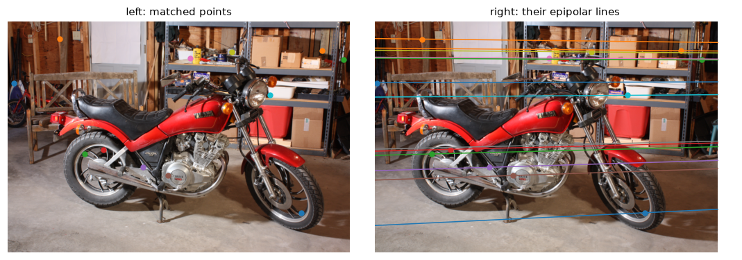 For a rectified pair, the fundamental matrix estimated from matches gives horizontal epipolar lines, and each matched point sits on its line: the correspondence search is along rows.
Matched points sit in the same row to about a tenth of a pixel. The estimated epipolar lines are within about a degree of horizontal, a looser check because a general \(\mathbf{F}\) has more freedom than the rectified geometry needs, and the epipole at infinity is poorly determined from noisy matches. Every dense stereo algorithm below relies on rectification: the match for left pixel \((x, y)\) is right pixel \((x - d, y)\).
Rectifying an unrectified pair
For the synthetic cameras, which are turned inward and not rectified, cv2.stereoRectify computes the rectifying rotations. Check that rectified matches end up in the same row:
R_rel, T_rel = R_true, t_true.reshape(3, 1)                  # X_2 = R X_1 + T
R1, R2, Pr1, Pr2, Q, _, _ = cv2.stereoRectify(K, None, K, None, (640, 480), R_rel, T_rel, alpha=0)
r1 = cv2.undistortPoints(x1.reshape(-1, 1, 2), K, None, R=R1, P=Pr1).reshape(-1, 2)
r2 = cv2.undistortPoints(x2.reshape(-1, 1, 2), K, None, R=R2, P=Pr2).reshape(-1, 2)
print(f"row difference before rectification: median {np.median(np.abs(x1[:, 1] - x2[:, 1])):.2f} px")
print(f"row difference after rectification:  median {np.median(np.abs(r1[:, 1] - r2[:, 1])):.2f} px")
print(f"rectified focal length {Pr1[0, 0]:.1f} px, baseline from P2: {-Pr2[0, 3] / Pr2[0, 0]:.3f} m")
row difference before rectification: median 16.62 px
row difference after rectification:  median 0.46 px
rectified focal length 917.8 px, baseline from P2: 0.500 m
After rectification the remaining row differences are just the 0.5-pixel noise, and the rectified projection matrices encode the baseline (\(\mathbf{P}_2\)'s fourth column is \(-fB\)).
Block matching from scratch, then StereoBM and StereoSGBM
A vectorized block matcher is short: for each candidate disparity \(d\), shift the right image by \(d\), take the absolute difference with the left image, and sum over a window with a box filter. That builds the cost volume one slice at a time. Winner-take-all picks the minimum. The evaluation uses the standard Middlebury-style metrics on pixels that have ground truth:
- Coverage: the fraction of GT pixels where the method returns a disparity at all.
- Bad-2.0 rate: among those, the fraction with an error above 2 pixels.
- MAE: the mean absolute disparity error among those.
import time

def evaluate(disp, name):
    has = (disp > 0) & valid_gt
    err = np.abs(disp - disp_gt)
    print(f"{name:22s} coverage {has.sum() / valid_gt.sum():6.1%}   bad-2.0 {np.mean(err[has] > 2):6.1%}"
          f"   MAE {err[has].mean():5.2f} px")

D = 64                                                       # disparities searched: 0..63
gLf, gRf = gl.astype(np.float32), gr.astype(np.float32)
Hh, Ww = gl.shape

def sad_cost_volume(gL, gR, D, win):
    C = np.full((D, *gL.shape), np.inf, np.float32)
    for d in range(D):
        diff = np.abs(gL[:, d:] - gR[:, :gL.shape[1] - d])   # left (x) vs right (x - d)
        C[d, :, d:] = cv2.boxFilter(diff, -1, (win, win))
    return C

t0 = time.perf_counter()
C_sad = sad_cost_volume(gLf, gRf, D, win=9)
disp_sad = C_sad.argmin(axis=0).astype(np.float32)
t_sad = time.perf_counter() - t0

t0 = time.perf_counter()
bm = cv2.StereoBM_create(numDisparities=64, blockSize=15)
disp_bm = bm.compute(gl, gr).astype(np.float32) / 16.0      # fixed point: 4 fractional bits
t_bm = time.perf_counter() - t0

bs = 5
t0 = time.perf_counter()
sgbm = cv2.StereoSGBM_create(minDisparity=0, numDisparities=64, blockSize=bs,
                             P1=8 * 3 * bs ** 2, P2=32 * 3 * bs ** 2, uniquenessRatio=10,
                             speckleWindowSize=100, speckleRange=2, disp12MaxDiff=1,
                             mode=cv2.STEREO_SGBM_MODE_SGBM_3WAY)
disp_sgbm = sgbm.compute(left, right).astype(np.float32) / 16.0
t_sgbm = time.perf_counter() - t0

evaluate(disp_sad, "SAD 9x9, from scratch")
evaluate(disp_bm, "cv2.StereoBM 15x15")
evaluate(disp_sgbm, "cv2.StereoSGBM")
print(f"time: SAD {t_sad * 1e3:.0f} ms, StereoBM {t_bm * 1e3:.0f} ms, StereoSGBM {t_sgbm * 1e3:.0f} ms")
SAD 9x9, from scratch  coverage  98.4%   bad-2.0  26.6%   MAE  4.22 px
cv2.StereoBM 15x15     coverage  78.4%   bad-2.0   6.9%   MAE  1.21 px
cv2.StereoSGBM         coverage  87.1%   bad-2.0   5.9%   MAE  1.00 px
time: SAD 159 ms, StereoBM 14 ms, StereoSGBM 19 ms
The raw winner-take-all SAD answers everywhere, and a quarter of its answers are wrong. StereoBM is much more accurate on the pixels it answers, mostly because it refuses to answer the hard ones: its prefilter, texture threshold, uniqueness ratio, and speckle filter remove about a fifth of the pixels. StereoSGBM is both more complete and more accurate. Always report coverage alongside error: a method that answers only the easy pixels can look excellent on error alone.
Common mistake: forgetting the factor of 16
StereoBM.compute and StereoSGBM.compute return int16 disparities in fixed point, multiplied by 16. Invalid pixels get (minDisparity - 1) * 16, which is \(-16\) here. Divide by 16.0 (as float) before using the values; treating the raw output as pixels makes every depth 16 times too small. Also: numDisparities must be a multiple of 16, and StereoBM needs single-channel 8-bit input.
Semi-global matching from scratch
Now the real thing. The data cost is the census transform (a 5 × 5 neighborhood, 24 bits per pixel) with Hamming distance, computed with NumPy 2's np.bitwise_count, lightly smoothed by a 3 × 3 box filter. Then aggregate along four paths with the SGM recursion and sum.
def census(img, r=2):
    """Census transform: one bit per neighbor in a (2r+1)^2 window, 1 if the neighbor is darker."""
    H_, W_ = img.shape
    p = np.pad(img, r, mode="edge")
    code = np.zeros((H_, W_), np.uint32)
    for dy in range(-r, r + 1):
        for dx in range(-r, r + 1):
            if dx or dy:
                code = (code << 1) | (p[r + dy:r + dy + H_, r + dx:r + dx + W_] < img).astype(np.uint32)
    return code

def census_cost_volume(gL, gR, D):
    cl, cr = census(gL), census(gR)
    C = np.full((D, *gL.shape), 24, np.float32)              # max Hamming distance where no match exists
    for d in range(D):
        C[d, :, d:] = np.bitwise_count(cl[:, d:] ^ cr[:, :gL.shape[1] - d])
    return np.stack([cv2.boxFilter(c, -1, (3, 3)) for c in C])

def sgm_path(C, P1, P2, axis, reverse):
    """Aggregate costs along one direction. C has shape (D, H, W); returns L_r with the same shape."""
    Cm = np.moveaxis(C, axis, 0)                              # (steps along the path, D, other)
    if reverse:
        Cm = Cm[::-1]
    L = np.empty_like(Cm)
    L[0] = Cm[0]
    inf_row = np.full((1, Cm.shape[2]), np.inf, np.float32)
    for i in range(1, len(Cm)):
        prev = L[i - 1]
        m = prev.min(axis=0, keepdims=True)
        plus = np.vstack([prev[1:], inf_row]) + P1          # came from d + 1
        minus = np.vstack([inf_row, prev[:-1]]) + P1        # came from d - 1
        L[i] = Cm[i] + np.minimum(np.minimum(prev, plus), np.minimum(minus, m + P2)) - m
    if reverse:
        L = L[::-1]
    return np.moveaxis(L, 0, axis)

t0 = time.perf_counter()
C_cen = census_cost_volume(gl, gr, D)
disp_census = C_cen.argmin(axis=0).astype(np.float32)
S = sum(sgm_path(C_cen, P1=8.0, P2=64.0, axis=ax, reverse=rev) for ax in (2, 1) for rev in (False, True))
disp_sgm = S.argmin(axis=0).astype(np.float32)
print(f"from-scratch census + SGM took {time.perf_counter() - t0:.1f} s")
evaluate(disp_census, "census WTA")
evaluate(disp_sgm, "census + SGM (4 paths)")

fig, axes = plt.subplots(2, 3, figsize=(10, 4.6))
panels = [(left, "left image"), (disp_gt, "ground truth"), (disp_sad, "SAD 9x9 (scratch)"),
          (disp_bm, "StereoBM"), (disp_sgm, "census + SGM (scratch)"), (disp_sgbm, "StereoSGBM")]
for ax, (im, title) in zip(axes.ravel(), panels):
    if im.ndim == 3:
        ax.imshow(im)
    else:
        ax.imshow(np.where(im > 0, im, np.nan), cmap="turbo", vmin=0, vmax=64)
    ax.set_title(title, fontsize=10); ax.axis("off")
plt.tight_layout(); plt.show()
from-scratch census + SGM took 1.8 s
census WTA             coverage  99.0%   bad-2.0  19.9%   MAE  3.76 px
census + SGM (4 paths) coverage  99.2%   bad-2.0  10.8%   MAE  2.25 px
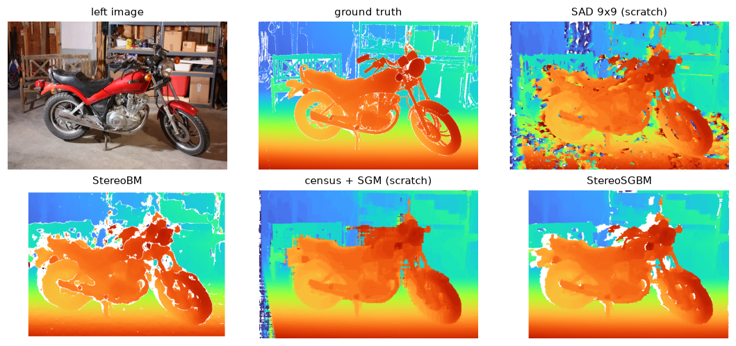 Ground truth and four estimates (white = no estimate). Winner-take-all SAD is noisy; StereoBM leaves holes; SGM aggregation smooths surfaces while keeping object boundaries.
The census cost alone is better than SAD; adding SGM's path aggregation halves the bad-pixel rate again, at nearly full coverage, without any post-filtering. OpenCV's StereoSGBM gets lower error partly by answering fewer pixels (its uniqueness, left-right, and speckle checks reject the doubtful ones), which is the next refinement you'd add (Exercise 4 does it).
From disparity to depth
Convert disparity to depth with the calibration from the dataset documentation, and compare depths directly. The depth error depends on distance, as the \(Z^2\) law says.
f_px, B_mm, doffs = 994.978, 193.001, 31.086

def to_depth(disp):
    return np.where(disp > 0, f_px * B_mm / (disp + doffs), np.nan)   # millimeters

Z_gt, Z_sgbm = to_depth(np.where(valid_gt, disp_gt, 0)), to_depth(disp_sgbm)
ok = valid_gt & (disp_sgbm > 0)
rel = np.abs(Z_sgbm[ok] - Z_gt[ok]) / Z_gt[ok]
print(f"GT depth range: {np.nanmin(Z_gt) / 1000:.2f} to {np.nanmax(Z_gt) / 1000:.2f} m")
print(f"StereoSGBM depth error: median {np.median(np.abs(Z_sgbm[ok] - Z_gt[ok])):.0f} mm,"
      f" median relative {np.median(rel):.2%}, share within 5%: {np.mean(rel < 0.05):.1%}")
for z_lo, z_hi in [(2000, 2500), (3000, 3500), (4000, 5100)]:
    band = ok & (Z_gt >= z_lo) & (Z_gt < z_hi)
    zc = (z_lo + z_hi) / 2
    print(f"  depth {z_lo / 1000:.1f}-{z_hi / 1000:.1f} m: median |error| {np.median(np.abs(Z_sgbm[band] - Z_gt[band])):6.0f} mm"
          f"   (Z^2/(fB) x 0.25 px = {zc ** 2 / (f_px * B_mm) * 0.25:4.0f} mm)")
GT depth range: 2.11 to 5.02 m
StereoSGBM depth error: median 7 mm, median relative 0.27%, share within 5%: 95.0%
  depth 2.0-2.5 m: median |error|      5 mm   (Z^2/(fB) x 0.25 px =    7 mm)
  depth 3.0-3.5 m: median |error|     13 mm   (Z^2/(fB) x 0.25 px =   14 mm)
  depth 4.0-5.1 m: median |error|     24 mm   (Z^2/(fB) x 0.25 px =   27 mm)
The scene spans about 2 to 5 m. The median depth error grows from about half a centimeter at 2 m to about 2.5 cm at 4–5 m, tracking \(Z^2/(fB)\) times a typical sub-pixel disparity error of about a quarter pixel (a little less, in fact: SGBM's median disparity error here is under 0.25 px).
Exercises
Exercise 1: Depth resolution by hand (easy)
A stereo camera has \(f = 1000\) px and \(B = 0.12\) m. (a) What depth corresponds to a disparity of 30 px? (b) If disparity is accurate to \(\pm 0.25\) px, what's the depth uncertainty there? (c) At what distance does the uncertainty reach 1 m? (d) What disparity range must the matcher search to cover depths from 1 m to infinity?
Solution
(a) \(Z = fB/d = 1000 \times 0.12 / 30 = 4\) m.
(b) \(\Delta Z = Z^2 \Delta d / (fB) = 16 \times 0.25 / 120 = 0.033\) m, about 3 cm.
(c) \(Z^2 = \Delta Z\,fB / \Delta d = 1 \times 120 / 0.25 = 480\), so \(Z \approx 21.9\) m.
(d) At 1 m, \(d = 120\) px; at infinity, \(d = 0\). The search range is 0–120, so numDisparities would be 128 (the next multiple of 16).
Exercise 2: Properties of E and F (easy)
Using E_true and F_true from the chapter: (a) verify numerically that the epipole \(\mathbf{e}_2\) (the null vector of \(\mathbf{F}^\top\)) is the projection of camera 1's center into image 2; (b) explain why \(\mathbf{F}\) has 7 degrees of freedom but \(\mathbf{E}\) only 5.
Solution
e2 = np.linalg.svd(F_true.T)[2][-1]
e2 = e2[:2] / e2[2]
c1_in_2 = project(P2, np.zeros((1, 3)))[0]                # camera 1's center is the world origin
print("epipole from F:", e2.round(2), "  camera 1 projected into camera 2:", c1_in_2.round(2))
The two agree. The epipole lies far outside the image (at \(x \approx 10{,}000\)) because the cameras are nearly side by side; for a perfectly rectified pair it would be at infinity. (b) \(\mathbf{F}\) is a general rank-2 \(3 \times 3\) matrix up to scale: \(9 - 1 - 1 = 7\). \(\mathbf{E} = [\mathbf{t}]_\times\mathbf{R}\) is built from a rotation (3) and a translation up to scale (2), so 5. Equivalently, \(\mathbf{E}\) must have two equal nonzero singular values, which adds two more constraints. Knowing \(\mathbf{K}\) is what removes the extra freedom.
Exercise 3: A planar scene breaks the eight-point algorithm (medium)
Generate 150 points on the plane \(Z = 6\) (with the same cameras and noise), build the eight-point matrix \(\mathbf{A}\) (normalized), and print its three smallest singular values. Compare with the non-planar scene in the chapter. Then estimate \(\mathbf{F}\) from the planar points and measure its epipolar distance on the non-planar points x1, x2. What do you conclude?
Solution
def eight_point_matrix(x1, x2):
    _, a = normalize_2d(x1); _, b = normalize_2d(x2)
    return np.column_stack([b[:, 0] * a[:, 0], b[:, 0] * a[:, 1], b[:, 0], b[:, 1] * a[:, 0],
                            b[:, 1] * a[:, 1], b[:, 1], a[:, 0], a[:, 1], np.ones(len(a))])

Xp = np.column_stack([rng.uniform(-1.5, 1.5, 150), rng.uniform(-1, 1, 150), np.full(150, 6.0)])
xp1 = project(P1, Xp) + rng.normal(0, 0.5, (150, 2))
xp2 = project(P2, Xp) + rng.normal(0, 0.5, (150, 2))
print("general scene, 3 smallest singular values:", np.linalg.svd(eight_point_matrix(x1, x2), compute_uv=False)[-3:].round(4))
print("planar scene,  3 smallest singular values:", np.linalg.svd(eight_point_matrix(xp1, xp2), compute_uv=False)[-3:].round(4))
F_plane = eight_point(xp1, xp2)
print(f"F from planar points: epipolar distance on its own points {epipolar_distance(F_plane, xp1, xp2).mean():.2f} px,"
      f" on the general scene {epipolar_distance(F_plane, x1, x2).mean():.1f} px")
general scene, 3 smallest singular values: [1.1706 1.0933 0.0574]
planar scene,  3 smallest singular values: [0.1061 0.0709 0.0625]
F from planar points: epipolar distance on its own points 0.51 px, on the general scene 12.5 px
For the general scene, only one singular value is near zero: a unique solution. For the plane, three singular values are at the noise level, so the null space is effectively three-dimensional, and the SVD picks an essentially arbitrary member. The resulting \(\mathbf{F}\) fits the planar matches perfectly but is wrong for the actual camera geometry (more than 10 pixels off on points off the plane). Points on one plane are related by a homography, which leaves \(\mathbf{F}\) underdetermined. Always check that your scene has depth variation, or fit a homography and compare.
Exercise 4: Left-right consistency (medium)
Occluded pixels have no true match, so any disparity assigned to them is wrong. Using the census cost volume C_cen (or the SGM sum S), compute the right image's disparity map from the same volume: for right pixel \((x_r, y)\), the cost of disparity \(d\) is \(C(d, y, x_r + d)\). Then keep a left pixel only if \(|d_L(x) - d_R(x - d_L(x))| \le 1\). Report coverage and bad-2.0 rate before and after the check.
Solution
def right_disparity(C):
    D_, H_, W_ = C.shape
    CR = np.full_like(C, np.inf)
    for d in range(D_):
        CR[d, :, :W_ - d] = C[d, :, d:]                   # right pixel x_r uses left pixel x_r + d
    return CR.argmin(axis=0)

def lr_check(dL, C, tol=1):
    dR = right_disparity(C)
    H_, W_ = dL.shape
    xs = np.arange(W_)[None, :] - dL.astype(int)
    inside = xs >= 0
    dR_at = np.take_along_axis(dR, np.clip(xs, 0, W_ - 1), axis=1)
    keep = inside & (np.abs(dL - dR_at) <= tol)
    return np.where(keep, dL, 0)

evaluate(disp_sgm, "SGM before LR check")
evaluate(lr_check(disp_sgm, S), "SGM after LR check")
SGM before LR check    coverage  99.2%   bad-2.0  10.8%   MAE  2.25 px
SGM after LR check     coverage  91.5%   bad-2.0   5.6%   MAE  1.19 px
The check removes about 8% of the pixels, mostly occlusions to the left of foreground objects and mismatches in dark, textureless regions, and cuts the bad-pixel rate roughly in half, to about the level of StereoSGBM (5.6% versus 5.9%) at higher coverage (91.5% versus 87.1%). Real pipelines then fill the holes (for example, with the smaller of the neighboring valid disparities, since occluded regions belong to the background).
Exercise 5: Sub-pixel disparity (hard)
Winner-take-all disparities are integers, so even a perfect match has up to 0.5 px of quantization error, which the depth formula amplifies. Implement parabola fitting: with costs \(c_-\), \(c_0\), \(c_+\) at \(d - 1\), \(d\), \(d + 1\), the minimum of the parabola through them is at
Derive this formula, apply it to the SGM sum S, and compare the MAE on pixels where the integer disparity is already within 1 px of the truth.
Solution
Fit \(c(\delta) = a\delta^2 + b\delta + c_0\) through \(\delta = -1, 0, 1\): \(c_- = a - b + c_0\) and \(c_+ = a + b + c_0\), so \(b = (c_+ - c_-)/2\) and \(a = (c_- - 2c_0 + c_+)/2\). The minimum is at \(\delta^* = -b/(2a) = (c_- - c_+)/(2(c_- - 2c_0 + c_+))\).
d0 = S.argmin(axis=0)
dd = np.clip(d0, 1, D - 2)
c_m = np.take_along_axis(S, (dd - 1)[None], 0)[0]
c_0 = np.take_along_axis(S, dd[None], 0)[0]
c_p = np.take_along_axis(S, (dd + 1)[None], 0)[0]
denom = c_m - 2 * c_0 + c_p
offset = np.where(denom > 0, (c_m - c_p) / (2 * np.maximum(denom, 1e-6)), 0)
disp_sub = dd + np.clip(offset, -0.5, 0.5)
near = valid_gt & (np.abs(d0 - disp_gt) <= 1)
print(f"integer WTA MAE on near-correct pixels: {np.abs(d0 - disp_gt)[near].mean():.3f} px")
print(f"sub-pixel MAE on the same pixels:       {np.abs(disp_sub - disp_gt)[near].mean():.3f} px")
Sub-pixel fitting helps, though less than you might hope: the integer error on these pixels is about 0.3 px, and fitting removes about a third of it. The SGM costs aren't exactly parabolic (the aggregation and the \(P_1\) penalty flatten them), and fitted offsets are biased toward integers ("pixel locking"). That's why StereoSGBM and learned stereo methods use more careful sub-pixel schemes.
Check yourself
-
What is an epipolar line, and why does it reduce the correspondence search from 2D to 1D?
Answer
It's the image in the second camera of the ray through the first camera's center and the pixel. The 3D point lies somewhere on that ray, so its projection in the second image must lie on the projected ray, a line. You only need to search along it.
-
Derive the epipolar constraint \(\hat{\mathbf{x}}_2^\top\mathbf{E}\hat{\mathbf{x}}_1 = 0\) in two sentences.
Answer
In camera 2's frame, the ray \(\hat{\mathbf{x}}_2\), the baseline \(\mathbf{t}\), and the rotated ray \(\mathbf{R}\hat{\mathbf{x}}_1\) all lie in the epipolar plane, so their triple product \(\hat{\mathbf{x}}_2^\top(\mathbf{t} \times \mathbf{R}\hat{\mathbf{x}}_1)\) is zero. Writing the cross product as \([\mathbf{t}]_\times\) gives \(\mathbf{E} = [\mathbf{t}]_\times\mathbf{R}\).
-
What's the difference between \(\mathbf{E}\) and \(\mathbf{F}\), and how many degrees of freedom does each have?
Answer
\(\mathbf{E}\) relates normalized (calibrated) coordinates and encodes only the relative pose: 5 degrees of freedom. \(\mathbf{F} = \mathbf{K}_2^{-\top}\mathbf{E}\mathbf{K}_1^{-1}\) relates pixel coordinates, absorbing the unknown intrinsics: 7 degrees of freedom.
-
Name the two steps that make the eight-point algorithm work in practice.
Answer
Hartley normalization of the points in each image before building the linear system, and enforcing rank 2 by zeroing the smallest singular value of the solution.
-
Why can't two calibrated views recover the length of the baseline?
Answer
The epipolar constraint is homogeneous in \(\mathbf{t}\): scaling the whole scene and the baseline together produces identical images. Only the translation direction is recoverable; the scale needs external information.
-
Derive \(Z = fB/d\), and explain why depth error grows with \(Z^2\).
Answer
In a rectified pair, \(x_L - c_x = fX/Z\) and \(x_R - c_x = f(X - B)/Z\); subtracting gives \(d = fB/Z\). Then \(|dZ/dd| = fB/d^2 = Z^2/(fB)\), so a fixed disparity error \(\Delta d\) causes a depth error \(\Delta Z \approx Z^2\Delta d/(fB)\).
-
Why does SGM outperform winner-take-all block matching in textureless regions?
Answer
Winner-take-all decides each pixel from its own window, which has no distinctive texture in such regions, so the minimum is essentially random. SGM adds smoothness penalties and aggregates costs along many 1D paths, so evidence from textured neighbors propagates into the textureless region, while the larger penalty \(P_2\) still permits real depth jumps.
-
What does bundle adjustment minimize, and over which variables?
Answer
The (robustified) sum of squared reprojection errors of all observed points in all images, jointly over all camera parameters (poses and possibly intrinsics) and all 3D point positions.
Key takeaways
- Two views are linked by the epipolar constraint: \(\hat{\mathbf{x}}_2^\top\mathbf{E}\hat{\mathbf{x}}_1 = 0\) with \(\mathbf{E} = [\mathbf{t}]_\times\mathbf{R}\) in normalized coordinates, and \(\tilde{\mathbf{u}}_2^\top\mathbf{F}\tilde{\mathbf{u}}_1 = 0\) with \(\mathbf{F} = \mathbf{K}_2^{-\top}\mathbf{E}\mathbf{K}_1^{-1}\) in pixels.
- The normalized eight-point algorithm (normalize, solve by SVD, enforce rank 2, denormalize), wrapped in RANSAC, estimates \(\mathbf{F}\). Planar scenes and pure rotations are degenerate.
- Decomposing \(\mathbf{E}\) gives four poses; the cheirality check picks one. The baseline's scale is unrecoverable without external information.
- Linear triangulation intersects rays by SVD; accuracy falls as rays become parallel.
- Rectified stereo turns matching into a 1D search along rows, and depth is \(Z = fB/d\) with error growing as \(Z^2/(fB)\).
- Block matching is fast but noisy and fattens edges; SGM aggregates costs along paths with smoothness penalties and is the practical classical standard. Always report coverage together with error.
Further reading
- R. Hartley and A. Zisserman, Multiple View Geometry in Computer Vision, 2nd ed., Cambridge University Press, 2004, chapters 9–12 (epipolar geometry, the fundamental matrix, and triangulation).
- R. Hartley, "In Defense of the Eight-Point Algorithm," IEEE Transactions on Pattern Analysis and Machine Intelligence, 19(6), 1997.
- H. Hirschmüller, "Stereo Processing by Semiglobal Matching and Mutual Information," IEEE Transactions on Pattern Analysis and Machine Intelligence, 30(2), 2008.
- D. Scharstein and R. Szeliski, "A Taxonomy and Evaluation of Dense Two-Frame Stereo Correspondence Algorithms," International Journal of Computer Vision, 47, 2002. The paper behind the Middlebury benchmark and the bad-pixel metric.
- J. L. Schönberger and J.-M. Frahm, "Structure-from-Motion Revisited," CVPR, 2016. The design of COLMAP.
Next
Stereo recovers depth from two cameras at one instant. The next chapter, Motion and tracking, uses one camera over time: optical flow, background subtraction, and tracking objects with Kalman filters.