Classical recognition

Level 2 · Chapter 6 · ⏱️ ~80 min read · Prerequisites: Features and keypoints, Edges and gradients, and the ML Handbook's chapters on SVMs and ensembles

Everything in this level so far has been about geometry: where things are and how they move. This chapter asks what they are. Before deep learning, recognition meant designing a feature by hand (a vector that summarizes an image region) and training a classical classifier on it. You'll build the most influential of these features: color histograms, Histograms of Oriented Gradients (implemented from scratch and matched against scikit-image), Local Binary Patterns, and bags of visual words. Then you'll turn a classifier into a detector with sliding windows and hard negative mining, classify faces with HOG and a linear SVM, and take apart the Viola-Jones face detector: integral images (implemented), Haar-like features, AdaBoost, and the attentional cascade. The chapter ends with why deep learning replaced these methods, and where they still win.

Why it matters

Wei joined a team that inspected wooden boards at a sawmill for knots and cracks. A previous contractor had trained a convolutional network on 400 labeled photos. It scored 97% on its validation set and about 70% on the production line. The validation photos came from the same afternoon as the training photos, and the network had partly learned the lighting of that afternoon.

Wei had a week and no budget for more labels. They computed Local Binary Pattern histograms on a grid of patches (a texture descriptor that, by construction, ignores any monotonic change in brightness), trained a linear SVM on the same 400 photos, and got 90% on the production line. It wasn't the final answer; the team later collected thousands of labeled images and a fine-tuned network overtook it. But for that week, a classical feature with the right invariance built in beat a model that had to learn its invariances from too little data.

Hand-crafted features are no longer the state of the art. They're still worth mastering, for three reasons: they're the right tool when data is tiny, compute is constrained, or decisions must be explained; every idea in them (gradient histograms, pooling, normalization, multi-scale search, cascades, hard negative mining) reappears inside modern detectors; and they make excellent baselines. If a network can't beat HOG plus an SVM, something is wrong.

Concepts

The classical recognition pipeline

A classical recognizer has two parts:

1. A feature extractor \(\phi\), designed by a person, that maps an image (or a window of one) to a fixed-length vector \(\phi(\mathbf{I}) \in \mathbb{R}^d\). It should keep what distinguishes the classes and discard what doesn't (lighting, small shifts, noise).
2. A classifier trained on those vectors: a linear SVM, logistic regression, a random forest, or boosted stumps.

The classifier is generic machine learning. The vision lies in \(\phi\). Every feature in this chapter makes deliberate choices about which invariances to build in, and, as you'll see, each invariance also throws information away.

Color histograms

The simplest global feature counts colors. Quantize each pixel's color into bins (for example 30 hue bins × 32 saturation bins in HSV, ignoring value so that brightness changes matter less), count, and normalize so the bins sum to 1. Compare two histograms \(\mathbf{h}\) and \(\mathbf{g}\) with:

• Histogram intersection \(\sum_i \min(h_i, g_i)\): 1 for identical histograms, 0 for disjoint ones (Swain and Ballard, 1991).
• Chi-squared distance \(\sum_i (h_i - g_i)^2 / (h_i + g_i)\), which weighs differences in rare bins more.
• Bhattacharyya distance, based on \(\sum_i \sqrt{h_i g_i}\).

A color histogram is invariant to translation, rotation, and flipping (it ignores where colors are), and fairly robust to partial occlusion and viewpoint changes. Its weakness is the same property: a red car and a red apple can have similar histograms. Color histograms are useful for image retrieval, tracking (as in mean-shift), and as one component of richer descriptors.

Histograms of Oriented Gradients

HOG (Dalal and Triggs, 2005) was designed for pedestrian detection and became the standard hand-crafted descriptor for object shape. The intuition: an object's shape is captured by the distribution of edge directions in local regions, and exact positions within each region don't matter much. A person's outline has strong vertical gradients at the sides of the torso and legs, and roughly horizontal ones at the shoulders and head.

The steps, for a detection window of \(64 \times 128\) pixels (the original pedestrian window):

1. Gradients. Compute \(g_x\) and \(g_y\) with the simple centered filter \([-1, 0, 1]\) (Dalal and Triggs found that larger, smoothed derivative filters such as Sobel performed worse: fine detail matters). Then the magnitude \(m = \sqrt{g_x^2 + g_y^2}\) and the unsigned orientation \(\theta = \operatorname{atan2}(g_y, g_x) \bmod 180°\). Unsigned means a dark-to-light edge and a light-to-dark edge at the same angle count the same, which suits people in clothes of any color against any background.
2. Cell histograms. Divide the window into cells of \(8 \times 8\) pixels. In each cell, build a histogram of orientations with 9 bins of 20°, each pixel voting with weight \(m\). (Dalal and Triggs split each vote between the two nearest bins and the four nearest cells by bilinear interpolation; scikit-image uses hard binning, as does the implementation below.)
3. Block normalization. Group cells into overlapping blocks of \(2 \times 2\) cells, sliding one cell at a time. Concatenate each block's four histograms (36 numbers) and normalize the vector. The L2-Hys scheme normalizes to unit L2 length, clips every entry at 0.2, and normalizes again, the same trick as SIFT's descriptor. Normalization over blocks makes the descriptor robust to local changes in contrast (a shadow over part of the person), and because blocks overlap, each cell appears in up to four differently normalized copies.
4. Concatenate all block vectors. For \(64 \times 128\): \(8 \times 16\) cells, \(7 \times 15\) block positions, \(105 \times 36 = 3{,}780\) dimensions.

HOG is invariant to small translations (within a cell), to local contrast changes (block normalization), and to the polarity of edges. It is not invariant to rotation or large scale changes: a person lying down has a different HOG. Detectors handle scale by searching an image pyramid, and simply don't handle rotation (people are usually upright).

Compare with SIFT. A SIFT descriptor is essentially a HOG-like histogram (\(4 \times 4\) cells, 8 bins) computed in a window rotated and scaled to a keypoint. HOG drops the keypoints and computes the same kind of descriptor densely on a fixed grid.

Local Binary Patterns

LBP (Ojala, Pietikäinen, and Harwood, 1996; Ojala et al., 2002) describes texture. For each pixel, compare its value with \(P\) neighbors on a circle of radius \(R\) (bilinearly interpolated where they fall between pixels), and write a 1 for each neighbor that is at least as bright as the center:

\[ \text{LBP}_{P,R}(\mathbf{x}) = \sum_{p=0}^{P-1} s\big(I(\mathbf{x}_p) - I(\mathbf{x})\big)\,2^p, \qquad s(z) = \begin{cases} 1 & z \ge 0 \\ 0 & z < 0. \end{cases} \]

With \(P = 8\) that's an 8-bit code, 256 possible values. The texture descriptor is the histogram of codes over a region.

Because only the signs of differences are used, LBP is invariant to any monotonic gray-level change: brightness, contrast, gamma. That's stronger than HOG's block normalization, and it's why Wei's sawmill model survived new lighting. Two refinements matter:

• Uniform patterns. A code is uniform if, read around the circle, it has at most two transitions between 0 and 1 (for example 00011100). Uniform codes correspond to edges, corners, line ends, and flat spots, and they account for the large majority of codes in natural images. Mapping all non-uniform codes to one bin gives 59 bins for \(P = 8\) (scikit-image's "nri_uniform").
• Rotation invariance. Rotating the image rotates each circular code. Mapping every code to the minimum over its circular rotations makes the histogram rotation-invariant. Combined with uniformity this leaves just \(P + 2 = 10\) bins: the number of 1s in a uniform code (0 to 8), plus one bin for non-uniform codes (scikit-image's "uniform", confusingly named).

LBP histograms computed on a grid of cells and concatenated were the state of the art for face recognition in the mid-2000s (Ahonen, Hadid, and Pietikäinen, 2006), and LBP is still used for texture classification and industrial inspection.

Bags of visual words

How do you get a fixed-length vector from a variable number of local descriptors (say, a few hundred SIFT descriptors per image)? Borrow an idea from text classification: describe a document by how often each word occurs, ignoring word order. The bag of visual words (BoVW, Sivic and Zisserman, 2003; Csurka et al., 2004):

1. Extract local descriptors from every training image, at keypoints or on a dense grid (dense usually works better for classification).
2. Build a vocabulary: cluster all descriptors with k-means into \(K\) clusters. Each cluster center is a visual word. (k-means is covered in the ML Handbook's clustering chapter.)
3. Encode each image: assign each of its descriptors to the nearest word and count, giving a \(K\)-bin histogram. Normalize it.
4. Classify the histograms with an SVM (a \(\chi^2\) or intersection kernel works best; a linear SVM after a square-root "Hellinger" mapping is a cheap approximation).

When the local descriptors are raw small patches, the words are called textons, a classic texture representation. Refinements fixed BoVW's main weaknesses: spatial pyramid matching (Lazebnik, Schmid, and Ponce, 2006) concatenates histograms over a \(1 \times 1\), \(2 \times 2\), and \(4 \times 4\) grid to restore coarse layout, and VLAD and Fisher vectors encode the residuals between descriptors and their words instead of just counts. BoVW with Fisher vectors was the best ImageNet method before AlexNet in 2012. And the vocabulary-plus-inverted-index structure still powers place recognition and loop closure in SLAM (for example DBoW2 in ORB-SLAM).

From classifier to detector: sliding windows

A classifier answers "is this window an X?". A detector answers "where are all the X's?". The classical bridge is the sliding window: classify a window at every position (with a stride of a few pixels) and at every scale. For scale, keep the window fixed and resize the image through a pyramid: an object twice the window's size becomes window-sized after downscaling by 2.

The cost is large. A \(640 \times 480\) image with a stride of 4 pixels has about 19,000 positions at full scale, and a pyramid with a factor of 1.2 adds about 2.3 times that. Tens of thousands of classifications per image is why the classifier must be cheap (linear) and why cascades matter.

Neighboring positions and scales overlap the same object, so a good detector fires many times around each true object. Non-maximum suppression (NMS) cleans this up: sort detections by score, keep the best, discard every other detection whose intersection over union (IoU, the area of the overlap divided by the area of the union) with it exceeds a threshold such as 0.3, and repeat. You'll meet IoU and NMS again in Level 4; every modern detector still uses them.

HOG + linear SVM, and hard negative mining

Dalal and Triggs's pedestrian detector is HOG features plus a linear SVM (a maximum-margin linear classifier, \(\hat{y} = \operatorname{sign}(\mathbf{w}^\top\phi(\mathbf{x}) + b)\); see the ML Handbook) scanned over a pyramid. Linear is essential for speed: the score is one dot product per window, and since \(\mathbf{w}\) has the same block structure as the HOG vector, it can even be visualized as a "template" of positive and negative gradient weights.

Positives are easy to collect (cropped, aligned examples), but what are the negatives? Almost every window in every image is a negative, far too many to train on, and almost all of them are trivially easy (sky, road). The fix is hard negative mining (also called bootstrapping):

1. Train on the positives and a random sample of negative windows.
2. Run the detector on images that contain no positives. Every detection is a false positive: a hard negative.
3. Add the hard negatives to the training set and retrain. Repeat once or twice.

This focuses the classifier's capacity on the confusing cases near the decision boundary. The same idea, under names like online hard example mining and focal loss, is central to training deep detectors.

Viola-Jones face detection

The Viola-Jones detector (2001) was the first real-time face detector, running at 15 frames per second on a 2001 laptop, and it powered the face boxes in point-and-shoot cameras for a decade. It combines four ideas.

Haar-like features. Each feature is the difference between the sums of pixels in adjacent rectangles: two rectangles side by side (an edge), three in a row (a line), or four in a checkerboard. On a face, the eye region is darker than the cheeks below it, and the bridge of the nose is brighter than the eyes on either side. In a \(24 \times 24\) window there are over 160,000 such features at all positions and sizes.

The integral image. Each feature needs rectangle sums, and computing them by adding pixels would be far too slow. The integral image (or summed-area table) stores at each position the sum of all pixels above and to the left:

\[ S(r, c) = \sum_{r' < r,\; c' < c} I(r', c'), \]

computed in one pass with two cumulative sums. Then the sum over any rectangle with top-left corner \((r_0, c_0)\) and size \(h \times w\) takes four lookups:

\[ \sum_{\text{rect}} I = S(r_0 + h, c_0 + w) - S(r_0, c_0 + w) - S(r_0 + h, c_0) + S(r_0, c_0). \]

Each Haar feature costs 6–9 array lookups regardless of its size, so a feature on a large window costs the same as on a small one, and scanning scales is done by scaling the features rather than the image.

AdaBoost feature selection. Most of the 160,000 features are useless. Viola and Jones used AdaBoost with decision stumps (a threshold on a single feature) as weak learners. Each boosting round picks the single feature and threshold with the lowest weighted error, then reweights the examples so the next round focuses on the mistakes. (AdaBoost is derived in the ML Handbook's ensembles chapter.) Boosting is simultaneously a feature selector and a classifier: 200 rounds give a strong classifier that looks at only 200 features. The first features chosen are exactly the intuitive ones: dark eyes above bright cheeks, a bright nose bridge between dark eyes.

The attentional cascade. Even 200 features per window is slow when nearly every window is a negative. The cascade is a sequence of increasingly complex boosted classifiers. Stage 1 uses two features and a threshold set so that it keeps nearly all faces (say 99.9%) while rejecting about half of the non-faces. Only windows that pass go to stage 2, and so on. The final detector had 38 stages and about 6,000 features, but the average window was evaluated on about 10 features, because most windows are rejected in the first two stages. If each stage has detection rate \(d_i\) and false positive rate \(f_i\), the cascade's overall rates are the products:

\[ D = \prod_{i=1}^{K} d_i, \qquad F = \prod_{i=1}^{K} f_i . \]

Ten stages with \(d_i = 0.99\) and \(f_i = 0.3\) give \(D \approx 0.90\) and \(F \approx 6 \times 10^{-6}\). The cascade structure, spend little computation on easy negatives and more on hard cases, reappears in two-stage detectors and in early-exit networks.

flowchart LR
    W["All windows"] --> S1{"Stage 1<br/>2 features"}
    S1 -->|reject ~50%| R["Not a face"]
    S1 -->|pass| S2{"Stage 2<br/>10 features"}
    S2 -->|reject ~80%| R
    S2 -->|pass| S3{"…"}
    S3 -->|reject| R
    S3 -->|pass all stages| F["Face"]

Viola-Jones detects frontal, upright faces well and fails on profiles, rotated faces, and strong occlusion; each pose needs its own cascade. Its lasting contributions are the integral image, boosting as feature selection, and cascades.

Why deep learning replaced hand-crafted features, and where they still win

In 2012, AlexNet cut the ImageNet top-5 error from about 26% (the best Fisher-vector system) to about 16%, and within three years learned features dominated every recognition benchmark. The reasons connect to everything above:

• Features are learned, not designed. HOG, LBP, and SIFT encode one person's guess of what matters. A network learns its features from data, for the task at hand, and the first layer of a trained CNN rediscovers oriented edge detectors and color blobs on its own. You'll see this in Level 3.
• Hierarchy. Hand-crafted pipelines have one or two levels of pooling. Deep networks stack many, building parts from edges and objects from parts.
• End-to-end training. In a classical pipeline the feature can't adapt to the classifier's errors. In a network, the loss gradient trains every layer.
• Scale of data and compute. Learned features need lots of data; ImageNet and GPUs supplied it.

Classical methods still win, or remain the sensible first choice, when:

• Data is tiny (tens to hundreds of images) and the needed invariance can be built in, as in Wei's sawmill.
• Compute is tiny: microcontrollers, battery-powered sensors, or very high frame rates.
• The problem is texture or geometry, not semantics: industrial surface inspection, document analysis, or anything where a fixed, well-understood response is needed.
• Explainability and certification matter: a HOG template or a threshold on an LBP histogram is easy to audit.
• As baselines, and as a check that a deep model isn't exploiting a shortcut.

In practice

Color histograms for retrieval

Compute hue-saturation histograms for a few images and compare a query (the left half of the cat photo) with candidates using intersection and the Bhattacharyya distance.

import time
import numpy as np
import cv2
import matplotlib.pyplot as plt
from skimage import data, feature
from sklearn.svm import LinearSVC
from sklearn.model_selection import cross_val_score, train_test_split

def hs_hist(img_rgb):
    """Normalized 30x32 hue-saturation histogram (value ignored)."""
    hsv = cv2.cvtColor(img_rgb, cv2.COLOR_RGB2HSV)
    h = cv2.calcHist([hsv], [0, 1], None, [30, 32], [0, 180, 0, 256])
    return h / h.sum()

cat = data.chelsea()
query = cat[:, :225]
candidates = {
    "cat, right half": cat[:, 225:],
    "cat, left half rotated + flipped": np.ascontiguousarray(np.flipud(np.rot90(query))),
    "cat, left half darkened 40%": (query * 0.6).astype(np.uint8),
    "coffee": data.coffee(),
    "rocket": data.rocket(),
    "astronaut": data.astronaut(),
}
hq = hs_hist(query)
print(f"{'candidate':34s} {'intersection':>12s} {'Bhattacharyya':>14s}")
for name, img in candidates.items():
    hc = hs_hist(img)
    inter = cv2.compareHist(hq, hc, cv2.HISTCMP_INTERSECT)
    bhat = cv2.compareHist(hq, hc, cv2.HISTCMP_BHATTACHARYYA)
    print(f"{name:34s} {inter:12.3f} {bhat:14.3f}")

candidate                          intersection  Bhattacharyya
cat, right half                           0.720          0.282
cat, left half rotated + flipped          1.000          0.000
cat, left half darkened 40%               0.981          0.055
coffee                                    0.356          0.649
rocket                                    0.074          0.863
astronaut                                 0.151          0.788

Rotation and flipping leave the histogram exactly unchanged. Darkening by 40% barely changes it, because the value channel is ignored; the small difference comes from 8-bit rounding, which shifts hue and saturation slightly in dark pixels. The other half of the same cat is the closest different image, and the coffee photo, with its warm browns, is closer than the blue rocket scene.

HOG from scratch, checked against scikit-image

The implementation follows scikit-image's conventions exactly: centered differences with zero gradient on the border row and column, unsigned orientation, hard binning, each cell's histogram divided by the cell area, and L2-Hys block normalization with \(\epsilon = 10^{-5}\).

def hog_scratch(img, orientations=9, cell=8, block=2, eps=1e-5):
    """HOG descriptor with scikit-image's conventions. Returns (feature vector, cell histograms)."""
    img = img.astype(np.float64)
    g_row, g_col = np.zeros_like(img), np.zeros_like(img)
    g_row[1:-1, :] = img[2:, :] - img[:-2, :]                 # [-1, 0, 1] filters
    g_col[:, 1:-1] = img[:, 2:] - img[:, :-2]
    mag = np.hypot(g_row, g_col)
    ang = np.rad2deg(np.arctan2(g_row, g_col)) % 180            # unsigned orientation
    bins = np.minimum((ang // (180 / orientations)).astype(int), orientations - 1)
    n_r, n_c = img.shape[0] // cell, img.shape[1] // cell
    hist = np.zeros((n_r, n_c, orientations))
    for i in range(n_r):
        for j in range(n_c):
            sl = np.s_[i * cell:(i + 1) * cell, j * cell:(j + 1) * cell]
            hist[i, j] = np.bincount(bins[sl].ravel(), weights=mag[sl].ravel(), minlength=orientations) / cell ** 2
    blocks = []
    for i in range(n_r - block + 1):
        for j in range(n_c - block + 1):
            v = hist[i:i + block, j:j + block].ravel()
            v = v / np.sqrt(np.sum(v ** 2) + eps ** 2)              # L2
            v = np.minimum(v, 0.2)                                  # clip ("Hys")
            v = v / np.sqrt(np.sum(v ** 2) + eps ** 2)              # renormalize
            blocks.append(v)
    return np.concatenate(blocks), hist

astro_gray = cv2.cvtColor(data.astronaut(), cv2.COLOR_RGB2GRAY)
person = cv2.resize(astro_gray[:, :256], (64, 128), interpolation=cv2.INTER_AREA) / 255.0   # a 64x128 "pedestrian" window
ours, cells = hog_scratch(person)
ref, hog_vis = feature.hog(person, orientations=9, pixels_per_cell=(8, 8), cells_per_block=(2, 2),
                           block_norm="L2-Hys", visualize=True)
print(f"descriptor length: ours {ours.size}, skimage {ref.size}  (= 7 x 15 blocks x 36)")
print(f"max |ours - skimage|: {np.abs(ours - ref).max():.1e}")

fig, axes = plt.subplots(1, 3, figsize=(7, 4.2))
axes[0].imshow(person, cmap="gray"); axes[0].set_title("64 x 128 window")
axes[1].imshow(hog_vis, cmap="gray"); axes[1].set_title("HOG cells")
axes[2].imshow(cells.argmax(axis=2) * 20, cmap="twilight", vmin=0, vmax=180); axes[2].set_title("dominant angle")
for ax in axes: ax.axis("off")
plt.tight_layout(); plt.show()

descriptor length: ours 3780, skimage 3780  (= 7 x 15 blocks x 36)
max |ours - skimage|: 5.6e-08

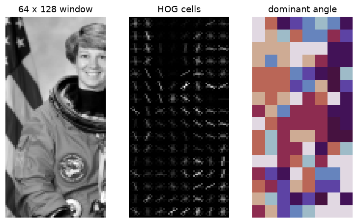HOG keeps one 9-bin orientation histogram per 8 × 8 cell. The visualization draws each bin as a line along the edge direction, weighted by its strength: the outline of the head, shoulders, and helmet survives, while the exact pixels don't.

The two agree to about \(10^{-8}\), and the length is the predicted 3,780.

Common mistake: HOG on images of different sizes

The HOG vector's length depends on the image size: \((n_{\text{cells,r}} - b + 1)(n_{\text{cells,c}} - b + 1)\,b^2\,n_{\text{bins}}\). Feeding windows of different sizes to one classifier fails with a shape error at best, or (if you pad or truncate vectors) silently compares unrelated blocks. Resize every window to the same size first, and keep the same pixels_per_cell, cells_per_block, and block_norm at training and test time.

Local Binary Patterns: texture, invariance, and its price

First, the operator itself. The implementation below samples \(P\) points on a circle of radius \(R\) with bilinear interpolation, following scikit-image's conventions (point \(p\) at angle \(2\pi p/P\), measured counterclockwise with rows pointing down, positions rounded to 5 decimals, zero padding).

def lbp_scratch(img, P=8, R=1.0, tol=1e-9):
    """'default' LBP codes with bilinear interpolation on a circle."""
    img = img.astype(np.float64)
    H_, W_ = img.shape
    theta = 2 * np.pi * np.arange(P) / P
    rp, cp = np.round(-R * np.sin(theta), 5), np.round(R * np.cos(theta), 5)
    rr, cc = np.mgrid[0:H_, 0:W_].astype(np.float64)
    pad = int(np.ceil(R)) + 1
    padded = np.pad(img, pad)
    code = np.zeros((H_, W_), np.int64)
    for p in range(P):
        r, c = rr + rp[p] + pad, cc + cp[p] + pad
        r0, c0 = np.floor(r).astype(int), np.floor(c).astype(int)
        fr, fc = r - r0, c - c0
        v = (padded[r0, c0] * (1 - fr) * (1 - fc) + padded[r0 + 1, c0] * fr * (1 - fc)
             + padded[r0, c0 + 1] * (1 - fr) * fc + padded[r0 + 1, c0 + 1] * fr * fc)
        code += ((v - img) >= -tol).astype(np.int64) << p      # tolerance absorbs rounding in near-ties
    return code

brick = data.brick()
codes_ours = lbp_scratch(brick)
codes_ref = feature.local_binary_pattern(brick, 8, 1, method="default")
print(f"LBP codes identical on {np.mean(codes_ours == codes_ref):.2%} of pixels")

LBP codes identical on 100.00% of pixels

The small tolerance matters. Without it, a few dozen pixels in this image disagree: an interpolated neighbor that should exactly equal the center comes out \(10^{-14}\) below it, and the \(\ge 0\) test flips.

Now classify textures. The three scikit-image textures (brick, grass, gravel) give 64 × 64 patches. To avoid leaking near-duplicate patches between training and test sets, training patches come only from the top half of each image and test patches only from the bottom half.

textures = {"brick": data.brick(), "grass": data.grass(), "gravel": data.gravel()}
trng = np.random.default_rng(0)

def random_crops(img, rows, n, size=64):
    out = []
    for _ in range(n):
        r = trng.integers(rows[0], rows[1] - size); c = trng.integers(0, img.shape[1] - size)
        out.append(img[r:r + size, c:c + size])
    return out

tex_train, tex_test, lab_train, lab_test = [], [], [], []
for k, img in enumerate(textures.values()):
    tex_train += random_crops(img, (0, 256), 60); lab_train += [k] * 60
    tex_test += random_crops(img, (256, 512), 40); lab_test += [k] * 40
lab_train, lab_test = np.array(lab_train), np.array(lab_test)

def lbp_hist(patch, method, P=8, R=1):
    codes = feature.local_binary_pattern(patch, P, R, method=method)
    n_bins = {"uniform": P + 2, "nri_uniform": P * (P - 1) + 3}[method]
    h, _ = np.histogram(codes, bins=n_bins, range=(0, n_bins))
    return h / h.sum()

for method in ["uniform", "nri_uniform"]:
    A = np.array([lbp_hist(p, method) for p in tex_train]); B = np.array([lbp_hist(p, method) for p in tex_test])
    clf = LinearSVC(C=10, max_iter=20000).fit(A, lab_train)
    dark = np.array([lbp_hist((p * 0.5).astype(np.uint8), method) for p in tex_test])   # half the brightness
    print(f"LBP {method:12s} ({A.shape[1]:2d} bins): test accuracy {clf.score(B, lab_test):.2f},"
          f" on darkened test patches {clf.score(dark, lab_test):.2f}")

LBP uniform      (10 bins): test accuracy 1.00, on darkened test patches 1.00
LBP nri_uniform  (59 bins): test accuracy 1.00, on darkened test patches 1.00

Both variants separate these textures perfectly, even after halving the brightness, which changes no comparison signs except through rounding. Now the price of invariance. Make a two-class problem: brick patches as they are versus brick patches rotated by 90° (horizontal versus vertical courses of bricks).

brick_tr, brick_te = random_crops(brick, (0, 256), 80), random_crops(brick, (256, 512), 50)
Xa = brick_tr[:40] + [np.rot90(p) for p in brick_tr[40:]]; ya = np.r_[np.zeros(40), np.ones(40)]
Xb = brick_te[:25] + [np.rot90(p) for p in brick_te[25:]]; yb = np.r_[np.zeros(25), np.ones(25)]
for method in ["uniform", "nri_uniform"]:
    A = np.array([lbp_hist(p, method) for p in Xa]); B = np.array([lbp_hist(p, method) for p in Xb])
    acc = LinearSVC(C=10, max_iter=20000).fit(A, ya).score(B, yb)
    print(f"horizontal vs vertical bricks, LBP {method:12s}: accuracy {acc:.2f}")

fig, axes = plt.subplots(2, 4, figsize=(10, 4.4))
for row, (name, img) in enumerate(list(textures.items())[:2]):
    patch = img[300:364, 300:364]
    axes[row, 0].imshow(patch, cmap="gray"); axes[row, 0].set_title(name, fontsize=9)
    axes[row, 1].imshow(feature.local_binary_pattern(patch, 8, 1, "uniform"), cmap="viridis")
    axes[row, 1].set_title("rotation-inv. uniform codes", fontsize=9)
    axes[row, 2].bar(range(10), lbp_hist(patch, "uniform")); axes[row, 2].set_title("10-bin histogram", fontsize=9)
    axes[row, 3].bar(range(59), lbp_hist(patch, "nri_uniform"), width=1.0); axes[row, 3].set_title("59-bin histogram", fontsize=9)
    for ax in axes[row, :2]: ax.axis("off")
plt.tight_layout(); plt.show()

horizontal vs vertical bricks, LBP uniform     : accuracy 0.44
horizontal vs vertical bricks, LBP nri_uniform : accuracy 1.00

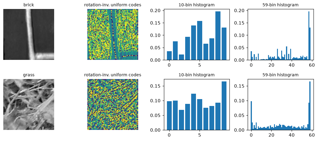LBP histograms of two textures. The 10-bin rotation-invariant histogram discards orientation; the 59-bin version keeps it.

The rotation-invariant descriptor is at chance: by design, it can't see orientation, so it can't tell horizontal bricks from vertical ones. The non-invariant version separates them perfectly. Every invariance you build in is information you throw away. Build in exactly the invariances your problem has, and no more.

Bag of visual words: the descriptor matters

Build a BoVW classifier for the same three textures. Each patch gets dense SIFT descriptors on a grid (every 4 pixels, 8-pixel keypoint size), a 100-word vocabulary comes from k-means on the training descriptors only, and each patch becomes a square-rooted, normalized word histogram for a linear SVM. As a second "dictionary", use textons: raw 7 × 7 patches with their mean subtracted and contrast normalized.

from sklearn.cluster import KMeans

sift = cv2.SIFT_create()
grid = [cv2.KeyPoint(float(x), float(y), 8) for y in range(8, 57, 4) for x in range(8, 57, 4)]
dense_sift = lambda p: sift.compute(p, grid)[1]

def raw_patches(p, s=7, step=3):
    p = p.astype(np.float32)
    out = np.array([p[r:r + s, c:c + s].ravel() for r in range(0, 64 - s, step) for c in range(0, 64 - s, step)])
    out -= out.mean(axis=1, keepdims=True)
    return out / (out.std(axis=1, keepdims=True) + 5)

def bovw_accuracy(describe, K=100):
    D_tr = [describe(p) for p in tex_train]; D_te = [describe(p) for p in tex_test]
    km = KMeans(K, random_state=0, n_init=2).fit(np.vstack(D_tr)[::2])     # vocabulary from training data only
    encode = lambda D: np.sqrt(np.bincount(km.predict(D), minlength=K) / len(D))
    A = np.array([encode(d) for d in D_tr]); B = np.array([encode(d) for d in D_te])
    clf = LinearSVC(C=1, max_iter=20000).fit(A, lab_train)
    return clf.score(B, lab_test), clf.predict(B)

t0 = time.perf_counter()
acc_sift, pred_sift = bovw_accuracy(dense_sift)
acc_tex, _ = bovw_accuracy(raw_patches)
print(f"BoVW with dense SIFT words: {acc_sift:.2f}   with texton words: {acc_tex:.2f}   ({time.perf_counter() - t0:.1f} s)")
from sklearn.metrics import confusion_matrix
print("dense-SIFT confusion matrix (rows: brick, grass, gravel):\n", confusion_matrix(lab_test, pred_sift))

BoVW with dense SIFT words: 0.78   with texton words: 1.00   (2.7 s)
dense-SIFT confusion matrix (rows: brick, grass, gravel):
 [[40  0  0]
 [ 0 24 16]
 [ 0 11 29]]

The pipeline is identical; only the local descriptor changed. SIFT words confuse grass with gravel, while texton words and LBP histograms separate all three. One likely reason: SIFT normalizes each descriptor to unit length and clips it, which discards exactly the local contrast and intensity statistics that distinguish these two random-looking textures, while it preserves gradient structure, which both have little of. SIFT words are the right choice for objects with distinctive parts; for stochastic textures, simpler descriptors that keep intensity statistics do better. This is the hand-crafted-feature workflow in a nutshell: the designer's guess about what matters decides the result.

HOG + linear SVM for faces vs non-faces

scikit-image's lfw_subset has 100 face crops and 100 non-face crops from the backgrounds of the same photos, each 25 × 25. Compare raw pixels, HOG (5 × 5 cells), and a grid of LBP histograms, each with a linear SVM and 5-fold cross-validation.

faces = data.lfw_subset()                                  # (200, 25, 25) floats in [0, 1]
y_face = np.r_[np.ones(100), np.zeros(100)]
hog_face = lambda im: feature.hog(im, orientations=9, pixels_per_cell=(5, 5), cells_per_block=(2, 2),
                                  block_norm="L2-Hys")

def lbp_grid(im, cells=5):
    codes = feature.local_binary_pattern((im * 255).astype(np.uint8), 8, 1, "nri_uniform")
    step = im.shape[0] // cells
    return np.concatenate([np.histogram(codes[i:i + step, j:j + step], bins=59, range=(0, 59))[0]
                           for i in range(0, cells * step, step) for j in range(0, cells * step, step)]) / step ** 2

feats = {"raw pixels": faces.reshape(200, -1),
         "HOG": np.array([hog_face(f) for f in faces]),
         "LBP grid": np.array([lbp_grid(f) for f in faces])}
for name, Xf in feats.items():
    scores = cross_val_score(LinearSVC(C=1.0, max_iter=20000), Xf, y_face, cv=5)
    print(f"{name:10s} {Xf.shape[1]:4d} dims   5-fold accuracy {scores.mean():.3f} ± {scores.std():.3f}")

raw pixels  625 dims   5-fold accuracy 0.945 ± 0.048
HOG         576 dims   5-fold accuracy 0.970 ± 0.019
LBP grid   1475 dims   5-fold accuracy 0.985 ± 0.012

On this small, clean dataset, raw pixels already reach about 95%, and the hand-crafted features are only a little better. These crops are aligned and evenly lit, so even a linear template on pixels works. The features earn their keep when the test images differ from the training images. Train on the original images, then test on copies that are darker (gamma 2), lower contrast, and shifted by 2 pixels:

idx_tr, idx_te = train_test_split(np.arange(200), test_size=0.3, random_state=0, stratify=y_face)

def perturb(im):
    im = 0.2 + 0.5 * im ** 2.0                                       # gamma 2 and lower contrast
    return np.roll(im, (2, 2), axis=(0, 1))                          # 2-pixel shift

perturbed = np.array([perturb(f) for f in faces])
extract = {"raw pixels": lambda ims: ims.reshape(len(ims), -1),
           "HOG": lambda ims: np.array([hog_face(f) for f in ims]),
           "LBP grid": lambda ims: np.array([lbp_grid(f) for f in ims])}
for name, fx in extract.items():
    clf = LinearSVC(C=1.0, max_iter=20000).fit(fx(faces[idx_tr]), y_face[idx_tr])
    print(f"{name:10s} clean test {clf.score(fx(faces[idx_te]), y_face[idx_te]):.2f}"
          f"   perturbed test {clf.score(fx(perturbed[idx_te]), y_face[idx_te]):.2f}")

raw pixels clean test 1.00   perturbed test 0.52
HOG        clean test 0.97   perturbed test 0.88
LBP grid   clean test 1.00   perturbed test 0.98

The pixel classifier collapses to chance: its decision depends on absolute brightness and exact positions. HOG and LBP lose much less, because gradient orientations and comparison signs barely change under a monotonic brightness change, and pooling over cells tolerates a small shift. This is the deal hand-crafted features offer: built-in invariance in exchange for flexibility.

A sliding-window detector with hard negative mining

To measure detection with exact ground truth, use a synthetic task: find upward-pointing triangles in cluttered scenes that also contain downward triangles, squares, and disks, in both light and dark versions, at sizes from 24 to 64 pixels. The window is 32 × 32 and is trained on triangles about 24 pixels across, so scales are searched with a pyramid.

WIN = 32
srng = np.random.default_rng(0)

def background(h, w):
    b = cv2.GaussianBlur(srng.normal(0, 1, (h, w)).astype(np.float32), (0, 0), 4)
    return 0.3 + 0.4 * (b - b.min()) / (b.max() - b.min())

def draw_shape(img, kind, cx, cy, s, val):
    if kind == "disk":
        cv2.circle(img, (int(cx), int(cy)), int(s * 0.45), val, -1, lineType=cv2.LINE_AA); return
    pts = {"tri_up": [[cx, cy - s / 2], [cx - s / 2, cy + s / 2], [cx + s / 2, cy + s / 2]],
           "tri_down": [[cx, cy + s / 2], [cx - s / 2, cy - s / 2], [cx + s / 2, cy - s / 2]],
           "square": [[cx - 0.4 * s, cy - 0.4 * s], [cx + 0.4 * s, cy - 0.4 * s],
                      [cx + 0.4 * s, cy + 0.4 * s], [cx - 0.4 * s, cy + 0.4 * s]]}[kind]
    cv2.fillPoly(img, [np.round(np.array(pts)).astype(np.int32)], val, lineType=cv2.LINE_AA)

def patch(kind, jitter=2.0, size=(20, 28), offset=(0, 0)):
    img = background(WIN, WIN)
    val = float(srng.choice([srng.uniform(0, 0.2), srng.uniform(0.8, 1.0)]))
    draw_shape(img, kind, WIN / 2 + offset[0] + srng.uniform(-jitter, jitter),
               WIN / 2 + offset[1] + srng.uniform(-jitter, jitter), srng.uniform(*size), val)
    return np.clip(img + srng.normal(0, 0.03, img.shape), 0, 1)

hog_win = lambda p: feature.hog(p, orientations=9, pixels_per_cell=(8, 8), cells_per_block=(2, 2), block_norm="L2-Hys")
positives = [patch("tri_up") for _ in range(400)]
negatives = [patch(k) for k in ["tri_down", "square", "disk"] for _ in range(150)]
negatives += [np.clip(background(WIN, WIN) + srng.normal(0, 0.03, (WIN, WIN)), 0, 1) for _ in range(200)]
negatives += [patch("tri_up", offset=srng.choice([-1, 1], 2) * srng.uniform(9, 14, 2)) for _ in range(150)]  # off-center
negatives += [patch("tri_up", size=(8, 12)) for _ in range(50)] + [patch("tri_up", size=(40, 50)) for _ in range(50)]
X_win = np.array([hog_win(p) for p in positives + negatives])
y_win = np.r_[np.ones(len(positives)), np.zeros(len(negatives))]
svm = LinearSVC(C=0.1, max_iter=20000).fit(X_win, y_win)
print(f"training windows: {len(positives)} positive, {len(negatives)} negative; HOG dims {X_win.shape[1]}")

training windows: 400 positive, 900 negative; HOG dims 324

The negatives deliberately include off-center and wrongly sized triangles, so the classifier learns to fire only when a triangle fills the window at the right scale. Now the scene, the scanner, NMS, and an evaluation that counts a detection as correct when its IoU with an unmatched ground-truth box is at least 0.5.

SH, SW = 300, 400

def make_scene(kinds):
    scene, placed, boxes = background(SH, SW), [], []
    for kind in kinds:
        for _ in range(200):
            s = srng.uniform(24, 64); cx = srng.uniform(s / 2 + 4, SW - s / 2 - 4); cy = srng.uniform(s / 2 + 4, SH - s / 2 - 4)
            if all(abs(cx - a) > (s + b) / 2 + 6 or abs(cy - c) > (s + b) / 2 + 6 for a, c, b in placed):
                break
        placed.append((cx, cy, s)); draw_shape(scene, kind, cx, cy, s, float(srng.choice([0.1, 0.9])))
        if kind == "tri_up":
            boxes.append((cx - s / 2, cy - s / 2, s, s))
    return np.clip(scene + srng.normal(0, 0.03, scene.shape), 0, 1), boxes

def box_iou(a, b):
    ax, ay, aw, ah = a; bx, by, bw, bh = b
    iw = max(0, min(ax + aw, bx + bw) - max(ax, bx)); ih = max(0, min(ay + ah, by + bh) - max(ay, by))
    return iw * ih / (aw * ah + bw * bh - iw * ih)

SCALES = 24 / np.geomspace(24, 64, 8)                      # resize so a triangle of size s becomes ~24 px

def sliding_window(img, clf, stride=4, thresh=0.0):
    """Returns (score, x, y, w, h) in original-image coordinates for windows scoring above thresh."""
    dets = []
    for s in SCALES:
        g = cv2.resize(img, None, fx=s, fy=s, interpolation=cv2.INTER_AREA)
        locs = [(c, r) for r in range(0, g.shape[0] - WIN + 1, stride) for c in range(0, g.shape[1] - WIN + 1, stride)]
        scores = clf.decision_function(np.array([hog_win(g[r:r + WIN, c:c + WIN]) for c, r in locs]))
        dets += [(v, (c + 4) / s, (r + 4) / s, 24 / s, 24 / s) for (c, r), v in zip(locs, scores) if v > thresh]
    return dets

def nms(dets, iou_thresh=0.3):
    keep = []
    for d in sorted(dets, key=lambda d: -d[0]):
        if all(box_iou(d[1:], k[1:]) < iou_thresh for k in keep):
            keep.append(d)
    return keep

def evaluate_dets(dets, gt_boxes):
    matched, tp = set(), 0
    for d in dets:
        ious = [box_iou(d[1:], g) for g in gt_boxes]
        j = int(np.argmax(ious))
        if ious[j] >= 0.5 and j not in matched:
            matched.add(j); tp += 1
    return tp, len(dets) - tp

test_scene, gt_boxes = make_scene(["tri_up"] * 5 + ["tri_down", "square", "disk"] * 3)
t0 = time.perf_counter()
raw = sliding_window(test_scene, svm)
dets_before = nms(raw)
tp, fp = evaluate_dets(dets_before, gt_boxes)
print(f"{len(raw)} windows above threshold -> {len(dets_before)} after NMS: {tp}/{len(gt_boxes)} found, {fp} false positives"
      f"  ({time.perf_counter() - t0:.1f} s)")

491 windows above threshold -> 43 after NMS: 5/5 found, 38 false positives  (3.8 s)

All five triangles are found, along with dozens of false positives on the distractor shapes and the textured background. Mine hard negatives: run the detector on two new scenes that contain no upward triangles, and add every window it fires on to the negatives.

hard = []
for _ in range(2):
    neg_scene, _ = make_scene(["tri_down", "square", "disk"] * 4)
    for v, x, yy, w, h in sliding_window(neg_scene, svm):
        s = 24 / w
        g = cv2.resize(neg_scene, None, fx=s, fy=s, interpolation=cv2.INTER_AREA)
        c, r = int(round(x * s - 4)), int(round(yy * s - 4))
        if g[r:r + WIN, c:c + WIN].shape == (WIN, WIN):
            hard.append(hog_win(g[r:r + WIN, c:c + WIN]))
svm2 = LinearSVC(C=0.1, max_iter=20000).fit(np.vstack([X_win, hard]), np.r_[y_win, np.zeros(len(hard))])
dets_after = nms(sliding_window(test_scene, svm2))
tp2, fp2 = evaluate_dets(dets_after, gt_boxes)
print(f"mined {len(hard)} hard negatives; after retraining: {tp2}/{len(gt_boxes)} found, {fp2} false positives")

fig, axes = plt.subplots(1, 2, figsize=(10, 3.9))
for ax, dets, title in zip(axes, [dets_before, dets_after], ["before hard negative mining", "after hard negative mining"]):
    ax.imshow(test_scene, cmap="gray", vmin=0, vmax=1)
    for g in gt_boxes:
        ax.add_patch(plt.Rectangle(g[:2], g[2], g[3], fill=False, ec="lime", lw=2))
    for v, x, yy, w, h in dets:
        ax.add_patch(plt.Rectangle((x, yy), w, h, fill=False, ec="red", lw=1))
    ax.set_title(title, fontsize=10); ax.axis("off")
plt.tight_layout(); plt.show()

mined 312 hard negatives; after retraining: 5/5 found, 8 false positives

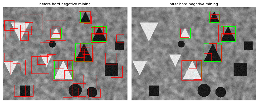Green: ground-truth upward triangles. Red: detections after NMS. One round of hard negative mining removes most false positives without losing any true detections.

One round of mining cuts the false positives by a factor of almost five while keeping every triangle. Most of the remaining false positives are smaller boxes on parts of the large triangles (a triangle's top half looks like a smaller triangle). NMS can't remove them, because a small box inside a large one has a low IoU with it; real detectors handle this with more mining rounds, part-aware training negatives, or an extra containment rule in NMS. Notice where the cost goes: scanning one 400 × 300 image takes seconds in Python, because HOG is recomputed for every overlapping window. Real implementations compute HOG once per pyramid level and score windows by sliding the SVM template over the grid of cells, which is the idea that later became "convolutional" sliding windows (OverFeat) and then fully convolutional detectors.

Common mistake: evaluating a detector on its training scenes

Hard negatives must come from images that are not in your test set, or the test numbers measure memorization. The same goes for the vocabulary in BoVW (fit k-means on training descriptors only) and for any threshold you tune. And split by source image, not by window: windows cut from one image are near-duplicates of each other.

Viola-Jones from the ground up: integral images, Haar features, boosting, cascades

The integral image takes two cumulative sums. OpenCV's cv2.integral returns the same table with an extra row and column of zeros, which makes the four-lookup formula work at the image border without special cases.

def integral(img):
    S = np.zeros((img.shape[0] + 1, img.shape[1] + 1), np.int64)
    S[1:, 1:] = img.astype(np.int64).cumsum(axis=0).cumsum(axis=1)
    return S

def rect_sum(S, r0, c0, h, w):
    return S[r0 + h, c0 + w] - S[r0, c0 + w] - S[r0 + h, c0] + S[r0, c0]

S = integral(astro_gray)
print("identical to cv2.integral:", np.array_equal(S, cv2.integral(astro_gray)))
irng = np.random.default_rng(0)
ok = True
for _ in range(1000):
    r0, c0 = irng.integers(0, 500, 2); h, w = irng.integers(1, 512 - max(r0, c0), 2)
    ok &= rect_sum(S, r0, c0, h, w) == astro_gray[r0:r0 + h, c0:c0 + w].astype(np.int64).sum()
print("1000 random rectangle sums match direct summation:", bool(ok))

big = np.random.default_rng(1).integers(0, 256, (2000, 2000), dtype=np.uint8)
S_big = integral(big)
t0 = time.perf_counter(); direct = [big[100:1900, 100:1900].sum() for _ in range(20)]; t_direct = (time.perf_counter() - t0) / 20
t0 = time.perf_counter(); fast = [rect_sum(S_big, 100, 100, 1800, 1800) for _ in range(20)]; t_fast = (time.perf_counter() - t0) / 20
print(f"1800x1800 rectangle: direct sum {t_direct * 1e3:.2f} ms, integral image {t_fast * 1e6:.1f} µs")

identical to cv2.integral: True
1000 random rectangle sums match direct summation: True
1800x1800 rectangle: direct sum 0.99 ms, integral image 0.9 µs

Now Haar-like features on the 25 × 25 face crops. scikit-image enumerates every feature of each type with haar_like_feature_coord (190,736 for five types in a 25 × 25 window) and evaluates them with haar_like_feature. Check one two-rectangle feature against a direct computation from its rectangle coordinates (for two-rectangle features, scikit-image's value is the second rectangle's sum minus the first's):

from skimage.transform import integral_image

feature_types = ["type-2-x", "type-2-y", "type-3-x", "type-3-y", "type-4"]
coords, types = feature.haar_like_feature_coord(25, 25, feature_types)
print(f"Haar-like features in a 25x25 window: {len(coords)}")

face0 = faces[0]
k = int(np.flatnonzero(types == "type-2-x")[500])
(r0a, c0a), (r1a, c1a) = coords[k][0]; (r0b, c0b), (r1b, c1b) = coords[k][1]
direct = face0[r0b:r1b + 1, c0b:c1b + 1].sum() - face0[r0a:r1a + 1, c0a:c1a + 1].sum()
lib = feature.haar_like_feature(integral_image(face0), 0, 0, 25, 25, feature_type=types[k:k + 1],
                                feature_coord=coords[k:k + 1])[0]
print(f"feature {k} ({types[k]}): direct {direct:.4f}, skimage {lib:.4f}")

Haar-like features in a 25x25 window: 190736
feature 500 (type-2-x): direct -1.8131, skimage -1.8131

Train an AdaBoost classifier with decision stumps on a random subset of 2,000 features. To make the cascade analysis meaningful, add 1,000 extra non-face crops (random 25 × 25 patches from other sample images), since real detectors see vastly more negatives than positives.

from sklearn.ensemble import AdaBoostClassifier
from sklearn.tree import DecisionTreeClassifier

hrng = np.random.default_rng(0)
sel = hrng.choice(len(coords), 2000, replace=False)
haar = lambda im: feature.haar_like_feature(integral_image(im), 0, 0, 25, 25,
                                            feature_type=types[sel], feature_coord=coords[sel])
extra_neg = []
for img in [data.coffee(), data.rocket(), data.brick(), data.grass(), data.gravel(), data.camera()]:
    g = (img if img.ndim == 2 else cv2.cvtColor(img, cv2.COLOR_RGB2GRAY)) / 255.0
    for s in [0.5, 0.25, 0.125]:
        gs = cv2.resize(g, None, fx=s, fy=s, interpolation=cv2.INTER_AREA)
        for _ in range(56):
            r, c = hrng.integers(0, gs.shape[0] - 25), hrng.integers(0, gs.shape[1] - 25)
            extra_neg.append(gs[r:r + 25, c:c + 25])
all_imgs = np.concatenate([faces, np.array(extra_neg)])
all_y = np.r_[y_face, np.zeros(len(extra_neg))]
t0 = time.perf_counter()
X_haar = np.array([haar(im) for im in all_imgs])
print(f"{len(all_imgs)} images ({int(all_y.sum())} faces), {X_haar.shape[1]} Haar features each,"
      f" computed in {time.perf_counter() - t0:.1f} s")

Xh_tr, Xh_rest, yh_tr, yh_rest = train_test_split(X_haar, all_y, test_size=0.5, random_state=0, stratify=all_y)
Xh_va, Xh_te, yh_va, yh_te = train_test_split(Xh_rest, yh_rest, test_size=0.5, random_state=0, stratify=yh_rest)
ada = AdaBoostClassifier(DecisionTreeClassifier(max_depth=1), n_estimators=50, random_state=0).fit(Xh_tr, yh_tr)
print(f"AdaBoost, 50 stumps: test accuracy {ada.score(Xh_te, yh_te):.3f}")

1208 images (100 faces), 2000 Haar features each, computed in 1.3 s
AdaBoost, 50 stumps: test accuracy 0.987

Each stump looks at exactly one feature, so the 50-round classifier uses at most 50 of the 2,000. Draw the first few it chose on a face:

chosen = [int(est.tree_.feature[0]) for est in ada.estimators_[:4]]
fig, axes = plt.subplots(1, 4, figsize=(8, 2.4))
for ax, j, rank in zip(axes, chosen, range(1, 5)):
    vis = feature.draw_haar_like_feature(faces[3], 0, 0, 25, 25, [coords[sel[j]]], max_n_features=1)
    ax.imshow(vis); ax.set_title(f"round {rank}: {types[sel[j]]}", fontsize=9); ax.axis("off")
plt.tight_layout(); plt.show()

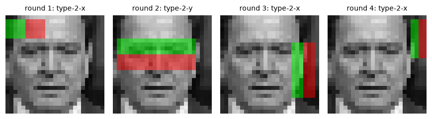The first features AdaBoost selected. Round 2 is the classic one: a band across the brows and eyes against the band below it. Others compare the edge of the face with the background beside it.

Finally, the cascade idea. AdaBoost's score after \(k\) rounds, \(\sum_{t \le k}\alpha_t h_t(\mathbf{x})\), is available from staged_decision_function. Treat the first \(k\) stumps as an early stage: set its threshold just low enough that every face in the validation split passes (thresholds set on training faces would be overfit, since boosting separates its own training data too well), and measure on the test split what fraction of faces survive and what fraction of non-faces the stage already rejects.

stage_sizes = [1, 2, 5, 10, 20, 50]
va_scores = list(ada.staged_decision_function(Xh_va))
te_scores = list(ada.staged_decision_function(Xh_te))
print(f"test split: {int(yh_te.sum())} faces, {int((yh_te == 0).sum())} non-faces")
print(f"{'stumps':>6s} {'faces kept':>11s} {'non-faces rejected':>19s}")
for k_st in stage_sizes:
    thr = va_scores[k_st - 1][yh_va == 1].min()           # keep every validation face
    keep = te_scores[k_st - 1] >= thr
    print(f"{k_st:6d} {keep[yh_te == 1].mean():11.2f} {1 - keep[yh_te == 0].mean():19.2f}")

test split: 25 faces, 277 non-faces
stumps  faces kept  non-faces rejected
     1        1.00                0.00
     2        0.92                0.91
     5        0.92                0.86
    10        1.00                0.91
    20        0.92                0.99
    50        1.00                0.99

A single stump can't reject anything: it has only two output values, and at least one validation face lands on the wrong side, so the threshold must let everything through. Two stumps already reject about 90% of the non-faces while keeping most faces (with only 25 test faces, each one is 4 points, so read the face column as rough). In a cascade, those rejected windows never reach the later, more expensive stages, so the average cost per window is a few features even though the full classifier uses many. That's the arithmetic behind Viola-Jones's real-time speed.

OpenCV 5 and the Haar cascade

OpenCV 4 shipped pretrained Viola-Jones cascades (haarcascade_frontalface_default.xml and others) and the Dalal-Triggs people detector (cv2.HOGDescriptor with getDefaultPeopleDetector). Check what this OpenCV 5 build provides:

import os
print("OpenCV", cv2.__version__)
print("cv2.CascadeClassifier available:", hasattr(cv2, "CascadeClassifier"))
print("cv2.HOGDescriptor available:   ", hasattr(cv2, "HOGDescriptor"))
print("bundled cascade XML files:", sorted(f for f in os.listdir(cv2.data.haarcascades) if f.endswith(".xml")))
print("cv2.FaceDetectorYN available:  ", hasattr(cv2, "FaceDetectorYN"))

OpenCV 5.0.0
cv2.CascadeClassifier available: False
cv2.HOGDescriptor available:    False
bundled cascade XML files: []
cv2.FaceDetectorYN available:   True

In OpenCV 5, the cascade classifier and the HOG people detector are no longer in the main package, and the pip build bundles no cascade files. The modern built-in face detector is cv2.FaceDetectorYN, a small CNN (YuNet) that needs an ONNX model file downloaded from the OpenCV model zoo. If you're on OpenCV 4.x, the classic API looks like this (not run here):

# OpenCV 4.x only: Viola-Jones face detection and the Dalal-Triggs people detector.
import cv2
img = cv2.imread("people.jpg")
gray = cv2.cvtColor(img, cv2.COLOR_BGR2GRAY)

cascade = cv2.CascadeClassifier(cv2.data.haarcascades + "haarcascade_frontalface_default.xml")
faces = cascade.detectMultiScale(gray, scaleFactor=1.1, minNeighbors=5, minSize=(30, 30))
for (x, y, w, h) in faces:                       # boxes are (x, y, w, h)
    cv2.rectangle(img, (x, y), (x + w, y + h), (0, 255, 0), 2)

hog = cv2.HOGDescriptor()                        # 64x128 window, 9 bins, 8x8 cells, 2x2 blocks
hog.setSVMDetector(cv2.HOGDescriptor_getDefaultPeopleDetector())
people, weights = hog.detectMultiScale(gray, winStride=(8, 8), padding=(8, 8), scale=1.05)

scaleFactor is the pyramid step (smaller is slower and finds more sizes), and minNeighbors is a crude NMS: a detection is kept only if at least that many overlapping raw detections support it. Raising it trades recall for precision.

Exercises

Exercise 1: HOG dimensions by hand (easy)

Compute the HOG descriptor length for (a) a \(64 \times 128\) window with 8-pixel cells, \(2 \times 2\) blocks, and 9 bins; (b) the same with \(16\)-pixel cells; (c) a \(25 \times 25\) face with 5-pixel cells, \(2 \times 2\) blocks, and 9 bins. Check (c) against the HOG features used for the faces above.

Solution

(a) \(8 \times 16\) cells, \(7 \times 15 = 105\) blocks, \(105 \times 4 \times 9 = 3{,}780\).

(b) \(4 \times 8\) cells, \(3 \times 7 = 21\) blocks, \(21 \times 36 = 756\).

(c) \(5 \times 5\) cells, \(4 \times 4 = 16\) blocks, \(16 \times 36 = 576\), which matches the 576 dimensions printed for HOG in the face experiment.

Exercise 2: Uniform patterns (easy)

Which of these 8-bit LBP codes are uniform: 00000000, 00111000, 01010000, 11100011, 10000001? Under scikit-image's rotation-invariant "uniform" mapping, which bin does each uniform code go to?

Solution

Count 0/1 transitions around the circle (including the wrap from the last bit back to the first):

• 00000000: 0 transitions, uniform, bin 0 (zero ones).
• 00111000: 2 transitions, uniform, bin 3.
• 01010000: 4 transitions, not uniform, goes to the shared bin \(P + 1 = 9\).
• 11100011: 2 transitions (the run of ones wraps around), uniform, bin 5.
• 10000001: 2 transitions (wrapping), uniform, bin 2.

The rotation-invariant uniform bin is simply the number of ones, because all rotations of a uniform pattern have the same number of ones and are therefore merged.

Exercise 3: The ratio of rejected windows in a cascade (medium)

A cascade has 10 stages, each with detection rate \(d = 0.995\) and false positive rate \(f = 0.4\). (a) What are the overall detection and false positive rates? (b) If stage \(i\) costs \(2i\) feature evaluations, what's the expected number of features evaluated for a non-face window? (c) For a face?

Solution

(a) \(D = 0.995^{10} \approx 0.951\); \(F = 0.4^{10} \approx 1.05 \times 10^{-4}\).

(b) A non-face reaches stage \(i\) with probability \(0.4^{i-1}\), so the expected cost is \(\sum_{i=1}^{10} 2i \cdot 0.4^{i-1}\).

(c) A face reaches stage \(i\) with probability \(0.995^{i-1}\), so the cost is close to the full \(\sum 2i = 110\).

cost_neg = sum(2 * i * 0.4 ** (i - 1) for i in range(1, 11))
cost_face = sum(2 * i * 0.995 ** (i - 1) for i in range(1, 11))
print(f"D = {0.995 ** 10:.3f}, F = {0.4 ** 10:.2e}, non-face cost {cost_neg:.2f}, face cost {cost_face:.1f}")

D = 0.951, F = 1.05e-04, non-face cost 5.55, face cost 106.7

Non-faces, which are nearly all windows, cost about 5.5 feature evaluations on average, 20 times less than a face. That asymmetry is the cascade's whole point.

Exercise 4: Spatial pyramid for BoVW (medium)

A plain bag of words ignores where words occur. Implement a two-level spatial pyramid for the dense-SIFT BoVW on textures: concatenate the whole-patch histogram with the four quadrant histograms (5 × 100 = 500 dimensions). Does it help on these textures? Explain why or why not.

Solution

pos = np.array([kp.pt for kp in grid])
quad = (pos[:, 1] >= 32).astype(int) * 2 + (pos[:, 0] >= 32).astype(int)   # quadrant of each grid point
D_tr = [dense_sift(p) for p in tex_train]; D_te = [dense_sift(p) for p in tex_test]
km = KMeans(100, random_state=0, n_init=2).fit(np.vstack(D_tr)[::2])

def spm(D):
    w = km.predict(D)
    hs = [np.bincount(w, minlength=100) / len(w)]
    hs += [np.bincount(w[quad == q], minlength=100) / max(1, np.sum(quad == q)) for q in range(4)]
    return np.sqrt(np.concatenate(hs))

A = np.array([spm(d) for d in D_tr]); B = np.array([spm(d) for d in D_te])
print(f"spatial pyramid BoVW accuracy: {LinearSVC(C=1, max_iter=20000).fit(A, lab_train).score(B, lab_test):.2f}")

spatial pyramid BoVW accuracy: 0.73

No improvement; it's slightly worse (0.73 versus 0.78). A spatial pyramid adds information about where words occur, which helps for scene and object categories with a typical layout (sky at the top, road at the bottom). Stationary textures look the same everywhere, so the quadrant histograms are just noisier copies of the global one, and the extra 400 dimensions give the SVM more room to fit noise. The confusion between grass and gravel comes from the SIFT descriptor itself, not from missing layout.

Exercise 5: The HOG + SVM template (hard)

A linear SVM on HOG features has a weight vector \(\mathbf{w}\) with the same structure as the descriptor (blocks × cells × bins). Reshape svm2.coef_ for the triangle detector into its \(3 \times 3\) blocks of \(2 \times 2\) cells and 9 bins, average the copies of each cell across the blocks that contain it, and display, for each of the \(4 \times 4\) cells, the orientation bin with the largest positive weight. Interpret the result in terms of the shape of an upward triangle.

Solution

w_blocks = svm2.coef_.reshape(3, 3, 2, 2, 9)                 # (block row, block col, cell row, cell col, bin)
w_cells, counts = np.zeros((4, 4, 9)), np.zeros((4, 4, 1))
for br in range(3):
    for bc in range(3):
        w_cells[br:br + 2, bc:bc + 2] += w_blocks[br, bc]; counts[br:br + 2, bc:bc + 2] += 1
w_cells /= counts
best_bin = w_cells.argmax(axis=2)
print("dominant positive orientation per cell (degrees of the gradient direction):")
print(best_bin * 20 + 10)

dominant positive orientation per cell (degrees of the gradient direction):
[[ 10  50 130 150]
 [110  50 130 110]
 [ 50  50 130 130]
 [ 50  90  90 130]]

These are gradient directions (perpendicular to edges), measured from the \(x\) axis with \(y\) pointing down. The bottom-middle cells favor 90° gradients, which belong to the triangle's horizontal base. Most cells in the left half favor gradients around 50° and most in the right half around 130°: oblique gradients of opposite tilt, the normals of the two slanted sides. A couple of cells (top left, for example) are noisy, since the triangle's apex and jittered position leave them little consistent structure. The SVM has learned a gradient template of an upward triangle, which is also why it learned to reject downward triangles, whose base is at the top. Dalal and Triggs's pedestrian template looks the same way: a person-shaped outline of weights.

Check yourself

1. What does block normalization do in HOG, and why do blocks overlap?

   Answer

   It normalizes each group of cells (to unit L2 norm, clipped at 0.2 and renormalized for L2-Hys), making the descriptor robust to local changes in illumination and contrast. Overlap means each cell is represented several times, normalized relative to different neighborhoods, which Dalal and Triggs found improves accuracy noticeably.

2. To what kind of intensity change is LBP invariant, and why?

   Answer

   Any monotonically increasing gray-level transformation (brightness, contrast, gamma), because each bit only records whether a neighbor is at least as bright as the center, and such transformations preserve that ordering.

3. Why did the rotation-invariant LBP fail to separate horizontal from vertical bricks?

   Answer

   Rotation invariance merges every code with its rotations, so the histogram no longer encodes orientation. The two classes differ only in orientation, so the descriptor can't see the difference. Each invariance discards information.

4. Describe the bag-of-visual-words pipeline in four steps.

   Answer

   Extract local descriptors (dense or at keypoints); cluster training descriptors with k-means into a vocabulary of \(K\) visual words; represent each image by its normalized histogram of nearest-word assignments; classify the histograms with an SVM (or another classifier).

5. What is hard negative mining, and why is it needed for sliding-window detectors?

   Answer

   Running the current detector on images without the target, collecting the false positives, adding them as negatives, and retraining. Nearly all windows are easy negatives; a random sample of them doesn't teach the classifier about the rare, confusing windows that cause false positives.

6. How does the integral image make Haar features fast, and what does a rectangle sum cost?

   Answer

   It stores cumulative sums so that any rectangle's sum is \(S(r_1, c_1) - S(r_0, c_1) - S(r_1, c_0) + S(r_0, c_0)\): four lookups and three additions, independent of the rectangle's size.

7. Why is a cascade so much faster than evaluating the full boosted classifier on every window?

   Answer

   The early stages are tiny and tuned to keep almost all faces while rejecting a large fraction of non-faces. Since almost every window is a non-face, most windows are rejected after a handful of features, and only the few promising windows pay for the full classifier.

8. Name three situations where a classical feature pipeline is still a reasonable choice today.

   Answer

   Very little labeled data with known invariances (for example, texture inspection under changing lighting); tight compute or power budgets (microcontrollers, very high frame rates); and when decisions must be auditable, or as a baseline and shortcut check for a deep model.

Key takeaways

• Classical recognition is a hand-designed feature plus a generic classifier; each feature builds in specific invariances and discards the information they ignore.
• Color histograms ignore layout; HOG pools gradient orientations into cells and normalizes over overlapping blocks; LBP encodes signs of local intensity differences and is invariant to monotonic lighting changes.
• Bags of visual words turn sets of local descriptors into fixed-length histograms over a k-means vocabulary; the choice of local descriptor can matter more than the classifier.
• Sliding windows plus an image pyramid turn a classifier into a detector; NMS removes duplicates, and hard negative mining fixes the flood of false positives.
• Viola-Jones combines Haar-like features, the integral image (constant-time rectangle sums), AdaBoost as feature selection, and an attentional cascade that spends computation only on promising windows.
• Deep learning replaced hand-crafted features by learning hierarchical features end to end, but classical methods still win with tiny data, tiny compute, or strict explainability, and remain essential baselines.

Further reading

• N. Dalal and B. Triggs, "Histograms of Oriented Gradients for Human Detection," CVPR, 2005.
• P. Viola and M. Jones, "Rapid Object Detection using a Boosted Cascade of Simple Features," CVPR, 2001; and "Robust Real-Time Face Detection," International Journal of Computer Vision, 57(2), 2004.
• T. Ojala, M. Pietikäinen, and T. Mäenpää, "Multiresolution Gray-Scale and Rotation Invariant Texture Classification with Local Binary Patterns," IEEE Transactions on Pattern Analysis and Machine Intelligence, 24(7), 2002.
• G. Csurka, C. Dance, L. Fan, J. Willamowski, and C. Bray, "Visual Categorization with Bags of Keypoints," ECCV Workshop on Statistical Learning in Computer Vision, 2004.
• S. Lazebnik, C. Schmid, and J. Ponce, "Beyond Bags of Features: Spatial Pyramid Matching for Recognizing Natural Scene Categories," CVPR, 2006.

Next

That completes the classical toolkit. Put the geometry half of it to work in the Level 2 capstone: stitch a panorama with your own RANSAC homographies and measure depth from stereo. Then move on to Level 3: CNNs for vision, where features stop being designed and start being learned.