Features and keypoints

Level 2 · Chapter 1 · ⏱️ ~75 min read · Prerequisites: Edges and gradients, Convolution and filtering, The frequency domain (for pyramids)

Before a computer can stitch two photos, track a drone, or recognize the same building from a different street corner, it has to find the same physical points in different images. This chapter covers how: what makes a point worth tracking, how to derive the Harris corner detector from first principles, how scale space lets you find blobs of any size, how SIFT and ORB turn a keypoint into a descriptor you can match, and how to measure whether all of this really survives rotation, scaling, and changes in lighting.

Why it matters

Priya's team built a shelf-auditing app for a grocery chain. A store clerk photographs a shelf with a phone, and the app matches the photo against a reference planogram image to check that every product sits where it should. In the lab, with photos taken square to the shelf at arm's length, it worked beautifully.

In the stores it failed on about one photo in three. The original matcher compared small fixed-size patches around corner points with plain pixel differences. A clerk who stepped back a meter made every product appear 30% smaller, so the patches no longer lined up. A clerk who tilted the phone rotated every patch. Under the warm fluorescent lights at the back of the store, every pixel was darker and more orange than in the reference photo, so the pixel differences were large even for perfect matches.

Swapping the patch matcher for SIFT keypoints with a ratio test, which you'll build up to in this chapter and the next, fixed nearly all of it in a day. The lesson wasn't "use SIFT". It was that a feature has to be designed for the changes it will actually face: scale, rotation, and lighting. Knowing how each detector achieves (or fails to achieve) each invariance is what lets you pick the right one and predict where it will break.

Concepts

What makes a good feature?

A feature (or keypoint, or interest point) is a location in an image that you can find again, reliably and precisely, in another image of the same scene. Three properties matter:

• Repeatability. If the same physical point is visible in two images, the detector should fire on it in both. Detection must not depend on the camera's position, rotation, zoom, or exposure.
• Distinctiveness. The neighborhood around the point should look different from the neighborhoods around other points, so that a match is unambiguous.
• Locality and precision. The point should be small (so occlusion or a change in viewpoint affects only a few features) and sharply localized (so you know exactly where it is).

Imagine sliding a small window across an image and asking, "If I move this window a little in any direction, does what I see change?" There are three cases.

• In a flat region (a patch of blue sky), moving the window in any direction changes nothing. You couldn't tell where you were.
• Along an edge (the boundary of a roof), moving the window along the edge changes nothing, while moving it across the edge changes a lot. You know your position in one direction but not the other. This is the aperture problem, which you'll meet again in Motion and tracking.
• At a corner (where two edges meet), moving the window in any direction changes what you see. Your position is pinned down in both directions.

Corners are the classic good feature: they're repeatable and precisely localized. Blobs (roughly round regions brighter or darker than their surroundings, like a coin, an eye, or a window pane) are the other classic: they have a natural center and, as you'll see, a natural size.

The Harris corner detector, derived

Let's turn the sliding-window intuition into math. Let \(I(x, y)\) be a grayscale image. Shift a window by \((u, v)\) and measure how much the content changes with the sum of squared differences (SSD), weighted by a window function \(w(x, y)\) (a box or a Gaussian centered on the point you're evaluating):

\[ E(u, v) = \sum_{x, y} w(x, y)\,\big[I(x + u, y + v) - I(x, y)\big]^2 . \]

A corner is a point where \(E(u, v)\) is large for every direction of the shift. A flat region has \(E \approx 0\) everywhere; an edge has \(E \approx 0\) along one direction.

For small shifts, use a first-order Taylor expansion. Write \(I_x = \partial I / \partial x\) and \(I_y = \partial I / \partial y\) for the image derivatives, which you computed with Sobel filters in Edges and gradients:

\[ I(x + u, y + v) \approx I(x, y) + I_x(x, y)\,u + I_y(x, y)\,v . \]

Substitute into \(E\):

\[ E(u, v) \approx \sum_{x, y} w(x, y)\,\big[I_x u + I_y v\big]^2 = \sum_{x, y} w(x, y)\,\big[I_x^2 u^2 + 2 I_x I_y\,uv + I_y^2 v^2\big]. \]

That is a quadratic form in \((u, v)\):

\[ E(u, v) \approx \begin{bmatrix} u & v \end{bmatrix} \mathbf{M} \begin{bmatrix} u \\ v \end{bmatrix}, \qquad \mathbf{M} = \sum_{x, y} w(x, y) \begin{bmatrix} I_x^2 & I_x I_y \\ I_x I_y & I_y^2 \end{bmatrix}. \]

The \(2 \times 2\) matrix \(\mathbf{M}\) is called the structure tensor (or second-moment matrix). It summarizes the distribution of gradient directions in the window. It's symmetric and positive semi-definite, so it has two real, non-negative eigenvalues \(\lambda_1 \ge \lambda_2 \ge 0\) with orthogonal eigenvectors \(\mathbf{e}_1, \mathbf{e}_2\).

The eigenvalues tell you everything. If you shift along eigenvector \(\mathbf{e}_i\) by distance \(t\), then \(E = \lambda_i t^2\). So \(\lambda_1\) is the change in the direction of fastest change, and \(\lambda_2\) is the change in the direction of slowest change. The level sets \(E(u, v) = c\) are ellipses with semi-axes proportional to \(\lambda_1^{-1/2}\) and \(\lambda_2^{-1/2}\).

Region	Eigenvalues	Why
Flat	\(\lambda_1 \approx \lambda_2 \approx 0\)	No gradients at all
Edge	\(\lambda_1 \gg \lambda_2 \approx 0\)	All gradients point the same way (across the edge)
Corner	\(\lambda_1 \ge \lambda_2 \gg 0\)	Strong gradients in two different directions

A corner is a point where the smaller eigenvalue is large. Shi and Tomasi (1994) use exactly that as the score: \(R_{\text{ST}} = \lambda_2 = \min(\lambda_1, \lambda_2)\). Harris and Stephens (1988) wanted to avoid computing eigenvalues, which for a \(2 \times 2\) matrix means a square root at every pixel (expensive in 1988). They noticed that the determinant and trace give the eigenvalues' product and sum for free:

\[ \det \mathbf{M} = \lambda_1 \lambda_2 = ac - b^2, \qquad \operatorname{tr} \mathbf{M} = \lambda_1 + \lambda_2 = a + c, \]

where \(a\), \(b\), \(c\) are the entries of \(\mathbf{M} = \begin{bmatrix} a & b \\ b & c \end{bmatrix}\). The Harris response is

\[ R = \det \mathbf{M} - k\,(\operatorname{tr} \mathbf{M})^2 = \lambda_1 \lambda_2 - k\,(\lambda_1 + \lambda_2)^2 , \]

with an empirical constant \(k\), usually between 0.04 and 0.06. Check the three cases:

• Flat: both eigenvalues near 0, so \(R \approx 0\).
• Edge: \(\lambda_2 \approx 0\), so \(R \approx -k \lambda_1^2 < 0\). Edges give negative responses.
• Corner: both large and comparable. With \(\lambda_1 = \lambda_2 = \lambda\), \(R = \lambda^2 (1 - 4k) > 0\).

So \(R > 0\) and large means corner. Why must \(k\) be small? Write \(\lambda_2 = r\lambda_1\) with \(0 \le r \le 1\). Then \(R = \lambda_1^2\,[r - k(1 + r)^2]\), which is positive only when \(r > k(1+r)^2\), roughly \(r > k\) for small \(k\). So \(k\) sets how "edge-like" (how lopsided) a structure can be and still count as a corner: a smaller \(k\) accepts more lopsided corners.

The full algorithm:

1. Compute \(I_x\) and \(I_y\) (Sobel), usually after light Gaussian smoothing.
2. Compute the three products \(I_x^2\), \(I_x I_y\), \(I_y^2\) at every pixel.
3. Sum each over the window: convolve with \(w\) (a box or a Gaussian of scale \(\sigma_I\), the integration scale). This gives \(a\), \(b\), \(c\) at every pixel.
4. Compute \(R = ac - b^2 - k(a + c)^2\).
5. Keep pixels where \(R\) is above a threshold (often a fraction of \(\max R\)) and is a local maximum (non-maximum suppression).

Two scales hide in Harris

The derivative scale \(\sigma_D\) (how much you smooth before differentiating) sets which details count as edges. The integration scale \(\sigma_I\) (the size of \(w\)) sets the size of the neighborhood whose gradients are pooled. Both are fixed in plain Harris, which is why it isn't scale-invariant.

What Harris is (and isn't) invariant to

Rotation. Rotate the image by a rotation matrix \(\mathbf{Q}\), and each gradient vector rotates by \(\mathbf{Q}\) too. The structure tensor becomes \(\mathbf{Q}\mathbf{M}\mathbf{Q}^\top\), which has the same eigenvalues. So the response \(R\) is unchanged at the corresponding point: Harris is rotation-invariant (up to small discretization effects from the square pixel grid and the square Sobel kernel).

Brightness offset. Adding a constant \(c\) to every pixel doesn't change any derivative, so \(R\) is unchanged.

Contrast (gain). Multiplying the image by \(g\) multiplies every gradient by \(g\), every entry of \(\mathbf{M}\) by \(g^2\), and \(R\) by \(g^4\). A fixed absolute threshold would therefore detect far fewer corners in a darker image. The usual fix is a relative threshold (like \(0.01 \max R\)), which is invariant to gain. Non-linear changes (gamma, a different white balance) are only approximately handled.

Scale. This is where Harris fails. Picture a rounded corner of a table. Zoomed out, it fits inside the window and looks like a corner. Zoomed in by a factor of 4, the window sees only a gently curving edge, with all gradients pointing almost the same way, so \(\lambda_2\) collapses and \(R\) goes negative. The same physical point is a corner at one scale and an edge at another. To handle zoom, you need the idea of scale space.

Scale space

The Gaussian scale space of an image is the family of blurred images

\[ L(x, y, \sigma) = G_\sigma * I, \qquad G_\sigma(x, y) = \frac{1}{2\pi\sigma^2} e^{-(x^2 + y^2)/(2\sigma^2)}, \]

for a continuous range of scales \(\sigma\). As \(\sigma\) grows, fine detail disappears and only coarse structure remains. Witkin (1983) and Koenderink (1984) showed that the Gaussian is the natural kernel for this: under reasonable axioms (linearity, shift invariance, and blurring never creating new structure), it's the only choice. You met a discrete version of this idea as the Gaussian pyramid in The frequency domain.

If an object appears twice as large in image B as in image A, then image B at scale \(2\sigma\) looks like image A at scale \(\sigma\) (up to the zoom). So if a detector can pick, for each feature, the scale at which it "looks best", that characteristic scale will grow proportionally with the object's size, and the feature can be described in a window proportional to it. That's the core trick of scale invariance: detect in position and scale together.

Blob detection with the scale-normalized Laplacian

What should "looks best" mean? Lindeberg (1998) proposed looking for extrema of normalized derivatives across scale. For blobs, the operator is the Laplacian of Gaussian (LoG), \(\nabla^2 L = L_{xx} + L_{yy}\), which you met as an edge detector in Level 1. Here it plays a different role: a LoG kernel looks like an upside-down Mexican hat, a dark center surrounded by a bright ring, so it responds strongly to a round blob of matching size.

There's a catch. Derivatives of a blurred image get weaker as you blur more (blurring spreads out intensity changes). A Gaussian derivative of order \(m\) shrinks by a factor of roughly \(\sigma^{-m}\), so the raw LoG response always decays with \(\sigma\) and you'd always pick the smallest scale. The fix is to multiply each derivative of order \(m\) by \(\sigma^m\). For the Laplacian (second order), the scale-normalized LoG is

\[ \nabla^2_{\text{norm}} L(x, y, \sigma) = \sigma^2\,\big(L_{xx} + L_{yy}\big). \]

Now take a disk of radius \(r\). Its normalized response at the center, as a function of \(\sigma\), rises, peaks, and falls. In 2D the peak occurs at

\[ \sigma^* = \frac{r}{\sqrt{2}}, \]

the scale at which the zero-crossing ring of the LoG kernel lines up with the disk's boundary. (The LoG kernel is zero on the circle \(x^2 + y^2 = 2\sigma^2\), so the ring has radius \(\sqrt{2}\sigma\).) A blob detector finds the points \((x, y, \sigma)\) that are local extrema of \(\sigma^2 |\nabla^2 L|\) in all three dimensions at once (comparing each sample with its 26 neighbors in a \(3 \times 3 \times 3\) cube), and reports a blob of radius \(\sqrt{2}\sigma\) there. You'll verify \(\sigma^* = r/\sqrt{2}\) numerically below.

Difference of Gaussians

Computing the LoG at many scales is expensive. Lowe's insight for SIFT was that the difference of Gaussians (DoG) approximates the scale-normalized LoG almost for free, because you're computing the blurred images anyway. The Gaussian satisfies the heat (diffusion) equation:

\[ \frac{\partial G_\sigma}{\partial \sigma} = \sigma\,\nabla^2 G_\sigma . \]

Approximate the derivative on the left with a finite difference between two nearby scales \(\sigma\) and \(k\sigma\):

\[ \frac{G_{k\sigma} - G_\sigma}{k\sigma - \sigma} \approx \sigma\,\nabla^2 G_\sigma \quad\Longrightarrow\quad G_{k\sigma} - G_\sigma \approx (k - 1)\,\sigma^2\,\nabla^2 G_\sigma . \]

The DoG is the scale-normalized LoG times the constant \((k - 1)\). Because the constant is the same at every scale, it doesn't move the extrema. So you build a stack of blurred images, subtract neighbors, and look for 3D extrema.

SIFT step by step

The Scale-Invariant Feature Transform (Lowe, 1999 and 2004) is the most influential feature pipeline in classical vision. It has two halves: a detector, which finds keypoints with a position, scale, and orientation; and a descriptor, which turns the neighborhood of each keypoint into a 128-number vector that you can compare between images.

flowchart LR
    A["Image"] --> B["Gaussian scale space<br/>(octaves × layers)"]
    B --> C["DoG images"]
    C --> D["3D extrema<br/>(26 neighbors)"]
    D --> E["Sub-pixel refinement,<br/>contrast and edge rejection"]
    E --> F["Dominant orientation(s)"]
    F --> G["128-D descriptor<br/>(4×4 cells × 8 bins)"]

1. Build the scale space. The image is blurred with a sequence of Gaussians. The scales are organized in octaves: each octave doubles \(\sigma\), and after each octave the image is downsampled by 2 (blurring by \(2\sigma\) at full resolution is equivalent to blurring by \(\sigma\) at half resolution, and much cheaper). Each octave has \(s\) intervals (Lowe used \(s = 3\)), so neighboring scales differ by \(k = 2^{1/s}\). Producing \(s\) usable DoG layers per octave requires \(s + 3\) blurred images. The base scale is \(\sigma_0 = 1.6\), and the input is usually upsampled by 2 first to keep the finest features.

2. Find extrema of the DoG. Each DoG sample is compared with its 8 neighbors at the same scale and the 9 + 9 at the scales above and below. Only samples larger (or smaller) than all 26 become candidates.

3. Refine and reject. A quadratic (second-order Taylor) fit of the DoG around each candidate gives a sub-pixel, sub-scale location. Then two filters remove unstable candidates:

• Low contrast. If the absolute DoG value at the refined extremum is small, the point is sensitive to noise, so it's dropped. (Lowe used 0.03 for images scaled to \([0, 1]\); OpenCV's contrastThreshold=0.04 is divided by the number of layers internally.)
• Edge responses. The DoG responds strongly along edges too, but such points are poorly localized along the edge, exactly the Harris problem. SIFT uses the \(2 \times 2\) Hessian \(\mathbf{H}\) of the DoG (second derivatives, not the structure tensor) and its eigenvalue ratio \(r = \lambda_1 / \lambda_2\). Since \(\operatorname{tr}(\mathbf{H})^2 / \det(\mathbf{H}) = (r + 1)^2 / r\) grows with \(r\), a point is kept only if \(\operatorname{tr}(\mathbf{H})^2 / \det(\mathbf{H}) < (r_{\max} + 1)^2 / r_{\max}\) with \(r_{\max} = 10\) (OpenCV's edgeThreshold=10). It's the same trick as Harris: use trace and determinant to avoid eigenvalues.

4. Assign an orientation. Around the keypoint, at its scale, SIFT computes gradient magnitudes and directions, and builds a 36-bin histogram of directions (10° each), weighted by magnitude and by a Gaussian of \(1.5\times\) the keypoint scale. The highest peak sets the keypoint's orientation. Any other peak within 80% of the highest creates an extra keypoint at the same place with that orientation (about 15% of keypoints get one).

5. Compute the descriptor. Take a window around the keypoint, sized proportional to its scale and rotated to its orientation. Divide it into a \(4 \times 4\) grid of cells. In each cell, build an 8-bin histogram of gradient directions (relative to the keypoint orientation), weighted by magnitude and by a Gaussian over the window, with trilinear interpolation between neighboring cells and bins so that small shifts don't cause jumps. That gives \(4 \times 4 \times 8 = 128\) numbers. Finally:

• Normalize the vector to unit length. This cancels a gain change in contrast, since gain scales all gradients equally. (An offset in brightness was already cancelled by using gradients.)
• Clip every entry at 0.2, then renormalize. Non-linear lighting changes (saturation, shading on 3D surfaces) mostly affect gradient magnitudes, not directions; clipping reduces the influence of a few very large gradients.

Every piece of invariance is now accounted for:

Change	How SIFT handles it
Translation	Keypoints are detected wherever the structure is
Scale	The characteristic scale from the DoG extremum; the descriptor window is sized by it
Rotation	The dominant orientation; the descriptor is computed in a rotated frame
Brightness offset	Gradients ignore constant offsets
Contrast (gain)	Unit-length normalization
Non-linear lighting	Clipping at 0.2 (approximately)
Small viewpoint change	Coarse spatial bins and histogramming tolerate small distortions

What SIFT doesn't handle well is large out-of-plane rotation (beyond roughly 40–50° of viewpoint change, the local patch distorts too much), strong blur, repeated texture (many keypoints look alike), and textureless surfaces (no keypoints at all).

SIFT's patent and OpenCV versions

SIFT was patented until March 2020. Older OpenCV builds exposed it only in the opencv-contrib package as cv2.xfeatures2d.SIFT_create. Since OpenCV 4.4 it's in the main package as cv2.SIFT_create, which is what this handbook uses with OpenCV 5. SURF (a faster SIFT relative) is still patented and only in contrib's "nonfree" build.

ORB and binary descriptors

SIFT descriptors are 128 floats compared by Euclidean distance. That's fine on a laptop and too slow for a phone tracking at 60 frames per second. ORB (Oriented FAST and Rotated BRIEF, Rublee et al., 2011) is a fast, free alternative that combines two earlier ideas and fixes their weaknesses.

FAST detection. FAST (Rosten and Drummond, 2006) examines the 16 pixels on a circle of radius 3 around a candidate pixel \(p\). If at least 9 contiguous pixels on the circle are all brighter than \(I(p) + t\) or all darker than \(I(p) - t\), for a threshold \(t\), then \(p\) is a corner. A quick pre-test on just 4 of the 16 pixels rejects most non-corners in a few comparisons, so FAST is extremely fast. But FAST also fires along edges and has no notion of orientation or scale. ORB fixes that:

• Ranking. ORB computes the Harris response at each FAST corner and keeps the top \(N\), which suppresses edge-like FAST responses.
• Scale. ORB runs FAST on an image pyramid (8 levels with a scale factor of 1.2 by default), so features are found at several scales. Unlike SIFT, there's no precise characteristic scale: each keypoint just takes the scale of the pyramid level where it was found.
• Orientation by intensity centroid. For a patch around the keypoint, compute the moments \(m_{pq} = \sum_{x, y} x^p y^q I(x, y)\) (with coordinates relative to the keypoint). The intensity centroid is at \((m_{10}/m_{00},\, m_{01}/m_{00})\), and the orientation is the direction from the keypoint to it: \(\theta = \operatorname{atan2}(m_{01}, m_{10})\). It's cheap, and it rotates exactly with the patch.

BRIEF description. A binary descriptor encodes a patch as a string of bits. BRIEF (Calonder et al., 2010) smooths the patch and then performs \(n = 256\) comparisons between pairs of pixel locations \((\mathbf{p}_i, \mathbf{q}_i)\) chosen in advance:

\[ b_i = \begin{cases} 1 & \text{if } I(\mathbf{p}_i) < I(\mathbf{q}_i) \\ 0 & \text{otherwise.} \end{cases} \]

The 256 bits pack into 32 bytes. Two descriptors are compared with the Hamming distance, the number of bits that differ, which a CPU computes with one XOR and a population-count instruction per 64 bits. That's tens of times faster than computing a 128-D Euclidean distance.

Because each bit is a comparison, a brightness offset or a gain change (anything that preserves the order of intensities) leaves BRIEF unchanged, which is more lighting invariance than SIFT's normalization. But plain BRIEF isn't rotation-invariant: rotate the patch and the pixel pairs land on different content. ORB's rBRIEF ("rotated BRIEF") rotates the sampling pattern by the keypoint's orientation \(\theta\) before comparing (they call this steered BRIEF), and chooses the 256 pairs by a greedy search on training data for tests that have high variance (each bit splits patches near 50/50) and low correlation with each other (each bit adds new information).

	SIFT	ORB
Detector	DoG extrema in scale space	FAST on a pyramid, ranked by Harris
Scale	Continuous characteristic scale	Pyramid level (discrete)
Orientation	Gradient histogram peak	Intensity centroid
Descriptor	128 floats (512 bytes)	256 bits (32 bytes)
Distance	Euclidean (L2)	Hamming
Speed	Slower	Roughly an order of magnitude faster
Typical use	Accurate matching, panoramas, 3D reconstruction	Real-time SLAM, mobile AR, video

Other binary descriptors (BRISK, FREAK) and floating-point ones (SURF, KAZE, AKAZE) fill in the design space between these two, and learned descriptors (SuperPoint, DISK, with matchers such as LightGlue) now beat all of them on hard viewpoint and lighting changes. You'll meet learned features in Level 3 and beyond. The ideas in this chapter (detect at a characteristic scale, normalize orientation, describe with pooled gradients) are what those networks learned to do better.

Testing invariance properly

Claims of invariance need a measurement. The standard protocol (Mikolajczyk and Schmid, 2005) uses image pairs related by a known transform \(\mathbf{H}\) (a homography, which you met in Geometric transformations). If you generate the second image yourself by warping the first, you know \(\mathbf{H}\) exactly. Then:

• Repeatability is the fraction of keypoints from image 1 (that land inside image 2 after mapping by \(\mathbf{H}\)) for which image 2 has a detected keypoint within a few pixels. It measures the detector alone.
• Matching precision is the fraction of descriptor matches whose image-1 point, mapped by \(\mathbf{H}\), lands within a few pixels of its matched image-2 point. It measures detector and descriptor together.

You'll use synthetic rotated, scaled, and relit versions of a real photo to measure both, which gives you ground truth for free.

In practice

Harris from scratch, checked against OpenCV

cv2.cornerHarris(src, blockSize, ksize, k) computes the response with a \(3 \times 3\) Sobel (for ksize=3) and an unnormalized box window of size blockSize. For a float image, OpenCV also scales the derivatives by \(1 / (2^{\text{ksize}-1} \cdot \text{blockSize})\). Knowing that, a from-scratch version can match it to floating-point precision.

import numpy as np
import cv2
import matplotlib.pyplot as plt
from skimage import data

def harris_response(img, block=3, ksize=3, k=0.04):
    """Harris response R = det(M) - k tr(M)^2, matching cv2.cornerHarris for float32 input."""
    img = img.astype(np.float32)
    scale = 1.0 / ((2 ** (ksize - 1)) * block)          # OpenCV's derivative scaling
    Ix = cv2.Sobel(img, cv2.CV_32F, 1, 0, ksize=ksize) * scale
    Iy = cv2.Sobel(img, cv2.CV_32F, 0, 1, ksize=ksize) * scale
    window = lambda a: cv2.boxFilter(a, -1, (block, block), normalize=False,
                                     borderType=cv2.BORDER_REFLECT_101)
    a, b, c = window(Ix * Ix), window(Ix * Iy), window(Iy * Iy)   # structure tensor entries
    return a * c - b * b - k * (a + c) ** 2

gray = cv2.cvtColor(data.chelsea(), cv2.COLOR_RGB2GRAY).astype(np.float32) / 255.0
R_ours = harris_response(gray, block=3, ksize=3, k=0.04)
R_cv = cv2.cornerHarris(gray, blockSize=3, ksize=3, k=0.04)
print("image shape:", gray.shape)
print(f"max |R|: {np.abs(R_cv).max():.3e}")
print(f"max abs difference: {np.abs(R_ours - R_cv).max():.3e}")

image shape: (300, 451)
max |R|: 7.343e-03
max abs difference: 9.313e-10

The two agree to about \(10^{-9}\), roughly single-precision rounding. The response map alone isn't a list of corners, though. You need a threshold and non-maximum suppression: a pixel is a corner if its \(R\) is above \(0.01 \max R\) and equal to the maximum in its \(5 \times 5\) neighborhood. Dilation (a max filter, from Morphology and classical segmentation) does the neighborhood maximum in one call.

def harris_corners(R, rel_thresh=0.01, nms_size=5):
    """Return (x, y) corners: above rel_thresh * max(R) and a local maximum."""
    local_max = cv2.dilate(R, np.ones((nms_size, nms_size), np.uint8))
    mask = (R == local_max) & (R > rel_thresh * R.max())
    ys, xs = np.nonzero(mask)
    return np.column_stack([xs, ys])

corners = harris_corners(R_ours)
print("corners found:", len(corners))

fig, axes = plt.subplots(1, 3, figsize=(10, 3.2))
axes[0].imshow(gray, cmap="gray"); axes[0].set_title("Input")
R_disp = np.sign(R_ours) * np.abs(R_ours) ** 0.25          # compress the range for display
axes[1].imshow(R_disp, cmap="coolwarm", vmin=-np.abs(R_disp).max(), vmax=np.abs(R_disp).max())
axes[1].set_title("Harris R (red > 0, blue < 0)")
axes[2].imshow(data.chelsea())
axes[2].scatter(corners[:, 0], corners[:, 1], s=8, c="yellow", edgecolors="black", linewidths=0.4)
axes[2].set_title(f"{len(corners)} corners after NMS")
for ax in axes: ax.axis("off")
plt.tight_layout(); plt.show()

corners found: 69

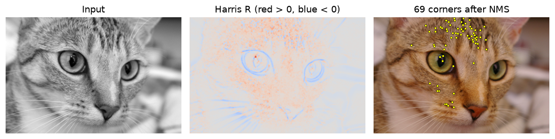The Harris response (fourth root for display): positive on corners such as the eyes and fur tips, negative along edges, near zero on smooth fur.

Common mistake: (x, y) versus (row, col)

np.nonzero returns (rows, cols), which is (y, x). OpenCV keypoints, cv2.circle, and matplotlib's scatter all expect (x, y). The column_stack([xs, ys]) above is deliberate. Swapping them gives corners mirrored across the diagonal, a bug that's easy to miss on square images.

Seeing the eigenvalues: flat, edge, and corner

The determinant-and-trace trick hides the eigenvalues. Computing them explicitly makes the three cases visible. For a symmetric \(2 \times 2\) matrix the eigenvalues have a closed form:

\[ \lambda_{1,2} = \frac{a + c}{2} \pm \sqrt{\left(\frac{a - c}{2}\right)^2 + b^2}. \]

The code below draws a synthetic scene with a rectangle, a triangle, and a disk, computes both eigenvalues with a Gaussian window, and labels each pixel.

def structure_tensor(img, sigma_d=1.0, sigma_i=2.0):
    """Entries (a, b, c) of the structure tensor with a Gaussian window."""
    sm = cv2.GaussianBlur(img, (0, 0), sigma_d)
    Ix = cv2.Sobel(sm, cv2.CV_32F, 1, 0, ksize=3)
    Iy = cv2.Sobel(sm, cv2.CV_32F, 0, 1, ksize=3)
    g = lambda x: cv2.GaussianBlur(x, (0, 0), sigma_i)
    return g(Ix * Ix), g(Ix * Iy), g(Iy * Iy)

scene = np.full((200, 300), 0.2, np.float32)
cv2.rectangle(scene, (30, 40), (120, 150), 0.9, -1)
cv2.fillPoly(scene, [np.array([[160, 160], [230, 40], [280, 170]])], 0.6)
cv2.circle(scene, (215, 120), 25, 0.1, -1)

a, b, c = structure_tensor(scene)
half_tr, root = (a + c) / 2, np.sqrt(((a - c) / 2) ** 2 + b ** 2)
lam1, lam2 = half_tr + root, half_tr - root
labels = np.zeros(scene.shape, np.uint8)                  # 0 = flat
labels[lam1 > 0.05 * lam1.max()] = 1                      # 1 = edge: one big eigenvalue
labels[lam2 > 0.05 * lam2.max()] = 2                      # 2 = corner: both big
print("pixels labeled flat / edge / corner:", np.bincount(labels.ravel(), minlength=3))

fig, axes = plt.subplots(1, 3, figsize=(10, 2.6))
axes[0].imshow(scene, cmap="gray", vmin=0, vmax=1); axes[0].set_title("Scene")
axes[1].imshow(lam2, cmap="magma"); axes[1].set_title(r"Smaller eigenvalue $\lambda_2$")
axes[2].imshow(labels, cmap=plt.matplotlib.colors.ListedColormap(["#222", "#4a90d9", "#f5a623"]))
axes[2].set_title("flat (black) / edge (blue) / corner (orange)")
for ax in axes: ax.axis("off")
plt.tight_layout(); plt.show()

pixels labeled flat / edge / corner: [51459  8061   480]

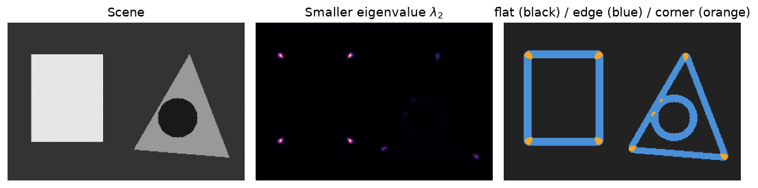Only the polygon corners, and the two junctions where the disk crosses the triangle's edge, have a large smaller eigenvalue. Straight edges and the disk's smooth boundary have one large eigenvalue and are labeled edges.

Notice the disk: its boundary curves, but over a window of a few pixels it's almost straight, so no point on it is a corner. Whether a curve is "a corner" depends on the window size relative to its curvature, which is the scale problem again.

Blob detection across scales

Now verify the scale-selection claim: for a disk of radius \(r\), the scale-normalized LoG response at the center peaks at \(\sigma^* = r/\sqrt{2}\). SciPy's ndimage.gaussian_laplace computes \(\nabla^2 (G_\sigma * I)\); multiply by \(\sigma^2\) to normalize, and negate so bright blobs give positive peaks.

from scipy import ndimage as ndi
from skimage import feature

blobs = np.zeros((120, 360), np.float32)
disks = [(60, 6), (170, 12), (290, 24)]                  # (center x, radius)
for cx, r in disks:
    cv2.circle(blobs, (cx, 60), r, 1.0, -1)

sigmas = np.geomspace(2, 30, 30)
stack = np.stack([-(s ** 2) * ndi.gaussian_laplace(blobs, s) for s in sigmas])   # (scales, H, W)
for cx, r in disks:
    s_best = sigmas[stack[:, 60, cx].argmax()]
    print(f"radius {r:2d}: best sigma {s_best:5.2f}   r/sqrt(2) = {r / np.sqrt(2):5.2f}")

found = feature.blob_log(blobs, min_sigma=2, max_sigma=30, num_sigma=30, threshold=0.1)
print("skimage blob_log (row, col, sigma):")
print(np.round(found, 2))

radius  6: best sigma  4.22   r/sqrt(2) =  4.24
radius 12: best sigma  8.12   r/sqrt(2) =  8.49
radius 24: best sigma 17.13   r/sqrt(2) = 16.97
skimage blob_log (row, col, sigma):
[[ 60.   290.    16.48]
 [ 60.   170.     8.76]
 [ 60.    60.     3.93]]

The best scales land on the nearest grid samples to \(r/\sqrt{2}\). scikit-image's blob_log finds the same three blobs at nearly the same scales (it uses a linear rather than geometric grid of sigmas, so its samples differ slightly). Plot the response curves and draw the detected blobs with radius \(\sqrt{2}\sigma\):

fig, axes = plt.subplots(1, 2, figsize=(10, 3), gridspec_kw={"width_ratios": [1, 1.6]})
for cx, r in disks:
    axes[0].plot(sigmas, stack[:, 60, cx], label=f"r = {r}")
    axes[0].axvline(r / np.sqrt(2), ls=":", c="gray")
axes[0].set_xlabel(r"$\sigma$"); axes[0].set_ylabel(r"$-\sigma^2 \nabla^2 L$ at center")
axes[0].legend(); axes[0].set_title("Scale-normalized LoG vs scale")
axes[1].imshow(blobs, cmap="gray")
for row, col, s in found:
    axes[1].add_patch(plt.Circle((col, row), np.sqrt(2) * s, color="orange", fill=False, lw=2))
axes[1].set_title(r"Detected blobs, radius $\sqrt{2}\,\sigma$"); axes[1].axis("off")
plt.tight_layout(); plt.show()

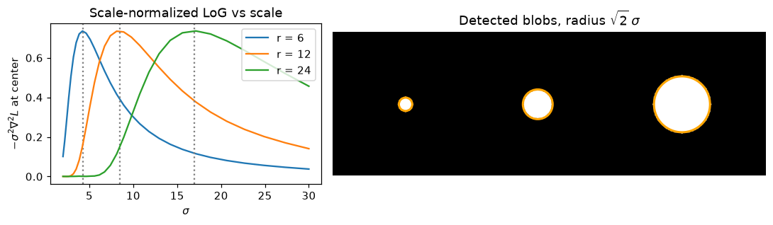Each disk's response peaks at its own characteristic scale (dotted lines at r/√2), so the detector recovers both where each blob is and how big it is.

This is the heart of scale invariance. If the image were zoomed by 2, each peak would move to twice the \(\sigma\), and a descriptor computed in a window proportional to \(\sigma\) would see the same content.

SIFT and ORB keypoints on a real image

OpenCV's detectors share one interface: detect, compute, or both at once with detectAndCompute(image, mask). Each keypoint carries pt (x, y), size (diameter of the meaningful neighborhood), angle (degrees), response (strength), and octave.

astro_rgb = data.astronaut()
astro = cv2.cvtColor(astro_rgb, cv2.COLOR_RGB2GRAY)

sift = cv2.SIFT_create()                      # defaults: nOctaveLayers=3, contrastThreshold=0.04, sigma=1.6
orb = cv2.ORB_create(nfeatures=1000)          # defaults: scaleFactor=1.2, nlevels=8, fastThreshold=20

kp_s, des_s = sift.detectAndCompute(astro, None)
kp_o, des_o = orb.detectAndCompute(astro, None)
print(f"SIFT: {len(kp_s)} keypoints, descriptors {des_s.shape} {des_s.dtype}")
print(f"ORB:  {len(kp_o)} keypoints, descriptors {des_o.shape} {des_o.dtype}")
k = kp_s[0]
print(f"one SIFT keypoint: pt=({k.pt[0]:.1f}, {k.pt[1]:.1f}) size={k.size:.1f} angle={k.angle:.1f}")
sizes = np.array([kp.size for kp in kp_s])
print(f"SIFT sizes: min {sizes.min():.1f}, median {np.median(sizes):.1f}, max {sizes.max():.1f}")
print("ORB descriptor bits set (first keypoint):", np.unpackbits(des_o[0]).sum(), "of 256")

flags = cv2.DRAW_MATCHES_FLAGS_DRAW_RICH_KEYPOINTS
vis_s = cv2.drawKeypoints(astro_rgb, kp_s[::4], None, color=(255, 200, 0), flags=flags)
vis_o = cv2.drawKeypoints(astro_rgb, kp_o[::4], None, color=(0, 255, 120), flags=flags)
fig, axes = plt.subplots(1, 2, figsize=(10, 5))
axes[0].imshow(vis_s); axes[0].set_title("SIFT (every 4th keypoint)")
axes[1].imshow(vis_o); axes[1].set_title("ORB (every 4th keypoint)")
for ax in axes: ax.axis("off")
plt.tight_layout(); plt.show()

SIFT: 1105 keypoints, descriptors (1105, 128) float32
ORB:  1000 keypoints, descriptors (1000, 32) uint8
one SIFT keypoint: pt=(4.7, 301.6) size=3.4 angle=139.5
SIFT sizes: min 1.8, median 3.3, max 80.7
ORB descriptor bits set (first keypoint): 135 of 256

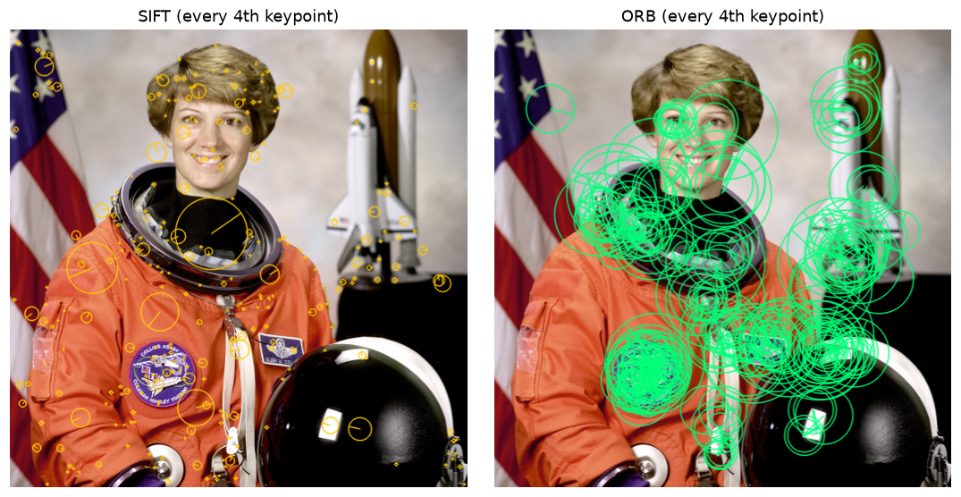Rich keypoints: each circle's radius is the keypoint scale and the line shows its orientation. SIFT spans a wide range of sizes; ORB's sizes come from its pyramid levels.

The image passed to drawKeypoints is RGB here, so the colors are given as RGB tuples too. With a BGR image from cv2.imread, the same tuple would draw a different color.

Common mistake: matching ORB descriptors with L2 distance

ORB descriptors are uint8 arrays of packed bits. If you match them with cv2.BFMatcher(cv2.NORM_L2), OpenCV happily computes Euclidean distances between the byte values, which are meaningless for bit strings. Always use cv2.NORM_HAMMING for ORB, BRIEF, BRISK, and AKAZE's binary descriptors, and cv2.NORM_L2 for SIFT.

Measuring invariance to rotation, scale, and lighting

Now test the invariance claims with ground truth. Make three versions of the astronaut image with known transforms: rotated by 30°, scaled by 0.6, and relit with a gamma of 1.8, a gain of 0.7, and an offset of 20. For each, detect and match with the ratio test (keep a match only if the best descriptor distance is under 0.75 times the second best; the next chapter explains why), and check every match against the true homography.

from scipy.spatial import cKDTree

h, w = astro.shape
M_rot = cv2.getRotationMatrix2D((w / 2, h / 2), 30, 1.0)       # 2x3 affine
variants = {
    "rotate 30°": (cv2.warpAffine(astro, M_rot, (w, h)), np.vstack([M_rot, [0, 0, 1]])),
    "scale 0.6": (cv2.resize(astro, None, fx=0.6, fy=0.6, interpolation=cv2.INTER_AREA),
                  np.diag([0.6, 0.6, 1.0])),
    "relight": (np.clip(255 * (astro / 255.0) ** 1.8 * 0.7 + 20, 0, 255).astype(np.uint8), np.eye(3)),
}

def map_points(pts, H):
    return cv2.perspectiveTransform(pts.reshape(-1, 1, 2).astype(np.float32), H).reshape(-1, 2)

def repeatability(pts1, pts2, H, shape, tol=3.0):
    """Fraction of image-1 points (that land inside image 2) with a detection within tol px."""
    proj = map_points(pts1, H)
    inside = (proj[:, 0] >= 0) & (proj[:, 0] < shape[1]) & (proj[:, 1] >= 0) & (proj[:, 1] < shape[0])
    dist, _ = cKDTree(pts2).query(proj[inside])
    return (dist < tol).mean()

def evaluate(detector, norm, img2, H, tol=3.0):
    k1, d1 = detector.detectAndCompute(astro, None)
    k2, d2 = detector.detectAndCompute(img2, None)
    p1 = np.float32([k.pt for k in k1]); p2 = np.float32([k.pt for k in k2])
    pairs = cv2.BFMatcher(norm).knnMatch(d1, d2, k=2)
    good = [m for m, n in pairs if m.distance < 0.75 * n.distance]
    q = p1[[m.queryIdx for m in good]]; t = p2[[m.trainIdx for m in good]]
    correct = np.linalg.norm(map_points(q, H) - t, axis=1) < tol
    return len(k2), repeatability(p1, p2, H, img2.shape, tol), len(good), correct.mean()

print(f"{'change':11s} {'method':5s} {'kp2':>5s} {'repeat':>7s} {'matches':>8s} {'precision':>9s}")
for name, (img2, H) in variants.items():
    for mname, det, norm in [("SIFT", cv2.SIFT_create(), cv2.NORM_L2),
                             ("ORB", cv2.ORB_create(1000), cv2.NORM_HAMMING)]:
        n2, rep, nm, prec = evaluate(det, norm, img2, H)
        print(f"{name:11s} {mname:5s} {n2:5d} {rep:7.2f} {nm:8d} {prec:9.2f}")

change      method   kp2  repeat  matches precision
rotate 30°  SIFT   1005    0.75      643      0.98
rotate 30°  ORB    1000    0.92      623      0.94
scale 0.6   SIFT    589    0.57      474      0.96
scale 0.6   ORB     920    0.95      417      0.98
relight     SIFT    725    0.54      526      0.96
relight     ORB    1000    0.85      513      0.95

Both pipelines keep their matches about 95% correct under all three changes. Read the other columns carefully, though:

• SIFT finds fewer keypoints after relighting (725 versus 1105). Its contrast threshold is absolute, and a gain of 0.7 plus a gamma of 1.8 compresses most of the image's contrast, so weak extrema fall below it. The descriptors are lighting-invariant; the detector's threshold isn't. ORB, capped at 1,000 keypoints and ranked by response, always returns its quota.
• ORB's repeatability looks higher, but part of that is density: 1,000 points in a \(512 \times 512\) image means a random point has a fair chance of having some detection within 3 pixels. Repeatability numbers are only comparable at similar keypoint densities. That's one reason benchmark papers fix the number of keypoints per image.
• Matching precision is the number that matters for the next chapter. Even 95% means 1 match in 20 is wrong, which is why every geometric estimate built on matches needs RANSAC.

Compare with plain Harris, which has no scale selection. Detect the top 500 Harris corners in the original and in each transformed image, and compute repeatability with a 2-pixel tolerance:

def harris_points(img, n=500):
    pts = cv2.goodFeaturesToTrack(img, maxCorners=n, qualityLevel=0.01, minDistance=5,
                                  useHarrisDetector=True, k=0.04)
    return pts.reshape(-1, 2)

p0 = harris_points(astro)
for name in ["rotate 30°", "scale 0.6"]:
    img2, H = variants[name]
    print(f"Harris repeatability, {name}: {repeatability(p0, harris_points(img2), H, img2.shape, tol=2):.2f}")

Harris repeatability, rotate 30°: 0.85
Harris repeatability, scale 0.6: 0.55

Harris is quite repeatable under rotation, as the eigenvalue argument predicts, and loses much of its repeatability when the image shrinks, because the fixed window now covers a different amount of the scene. Finally, look at SIFT matches on a harder pair that combines rotation, scaling, and a lighting change:

M_hard = cv2.getRotationMatrix2D((w / 2, h / 2), 40, 0.7)
hard = cv2.warpAffine(astro, M_hard, (w, h))
hard = np.clip(hard.astype(np.float32) * 0.6 + 30, 0, 255).astype(np.uint8)
H_hard = np.vstack([M_hard, [0, 0, 1]])

k1, d1 = sift.detectAndCompute(astro, None)
k2, d2 = sift.detectAndCompute(hard, None)
good = [m for m, n in cv2.BFMatcher(cv2.NORM_L2).knnMatch(d1, d2, k=2) if m.distance < 0.75 * n.distance]
q = np.float32([k1[m.queryIdx].pt for m in good]); t = np.float32([k2[m.trainIdx].pt for m in good])
ok = np.linalg.norm(map_points(q, H_hard) - t, axis=1) < 3
print(f"{len(good)} ratio-test matches, {ok.mean():.1%} correct")

sample = good[::8]
vis = cv2.drawMatches(astro, k1, hard, k2, sample, None,
                      matchColor=(0, 200, 255), flags=cv2.DRAW_MATCHES_FLAGS_NOT_DRAW_SINGLE_POINTS)
plt.figure(figsize=(10, 4.2)); plt.imshow(vis); plt.axis("off")
plt.title("SIFT matches under rotation 40°, scale 0.7, and gain/offset (every 8th match)")
plt.tight_layout(); plt.show()

394 ratio-test matches, 93.9% correct

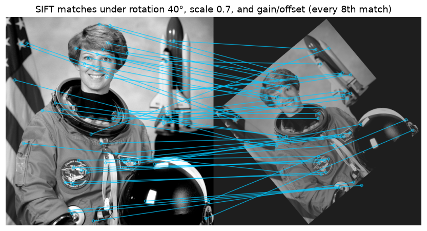Nearly all lines connect the same physical points despite the combined rotation, zoom, and lighting change.

Common mistake: feeding color or float images to detectors

detectAndCompute expects an 8-bit image. SIFT and ORB convert a 3-channel input to grayscale internally (assuming BGR order), but float images in \([0, 1]\) will either be rejected or behave as if they were nearly black, because thresholds such as ORB's fastThreshold=20 are in 0–255 units. Convert to uint8 grayscale yourself, so you control the conversion.

Exercises

Exercise 1: Harris by hand (easy)

At three pixels, the structure tensor (after windowing) is:

• (a) \(\mathbf{M} = \begin{bmatrix} 10 & 0 \\ 0 & 0.1 \end{bmatrix}\)
• (b) \(\mathbf{M} = \begin{bmatrix} 5 & 4 \\ 4 & 5 \end{bmatrix}\)
• (c) \(\mathbf{M} = \begin{bmatrix} 6 & 0 \\ 0 & 5 \end{bmatrix}\)

For each, compute the eigenvalues, the Harris response with \(k = 0.05\), and the Shi-Tomasi score. Classify each pixel as flat, edge, or corner. Which pixel would a corner detector consider strongest?

Solution

(a) The matrix is diagonal, so \(\lambda_1 = 10\), \(\lambda_2 = 0.1\). \(\det = 1\), \(\operatorname{tr} = 10.1\), \(R = 1 - 0.05 \times 102.01 = -4.10\). Shi-Tomasi: 0.1. Negative \(R\) and one dominant eigenvalue: an edge (a vertical one, since the large eigenvalue belongs to \(x\): gradients point along \(x\)).

(b) Eigenvalues of \(\begin{bmatrix} a & b \\ b & a \end{bmatrix}\) are \(a \pm b\): \(\lambda_1 = 9\), \(\lambda_2 = 1\). \(\det = 25 - 16 = 9\), \(\operatorname{tr} = 10\), \(R = 9 - 0.05 \times 100 = 4\). Shi-Tomasi: 1. Positive but with a 9:1 ratio: a weak corner, or a diagonal edge with some texture. The off-diagonal term means the dominant gradient direction is diagonal (\(\mathbf{e}_1 \propto (1, 1)\)).

(c) \(\lambda_1 = 6\), \(\lambda_2 = 5\). \(\det = 30\), \(\operatorname{tr} = 11\), \(R = 30 - 0.05 \times 121 = 23.95\). Shi-Tomasi: 5. Strong gradients in both directions: a corner, and the strongest of the three by both scores.

A quick NumPy check:

for M in [np.array([[10, 0], [0, 0.1]]), np.array([[5, 4], [4, 5]]), np.array([[6, 0], [0, 5]])]:
    lam = np.linalg.eigvalsh(M)[::-1]
    R = np.linalg.det(M) - 0.05 * np.trace(M) ** 2
    print(f"eigenvalues {lam.round(2)}, Harris R = {R:.2f}, Shi-Tomasi = {lam[1]:.2f}")

eigenvalues [10.   0.1], Harris R = -4.10, Shi-Tomasi = 0.10
eigenvalues [9. 1.], Harris R = 4.00, Shi-Tomasi = 1.00
eigenvalues [6. 5.], Harris R = 23.95, Shi-Tomasi = 5.00

Exercise 2: How Harris scales with contrast (easy)

Without running code, predict: if you multiply an image by 0.5 (halve its contrast), by what factor does the Harris response \(R\) change at every pixel? Why does cv2.goodFeaturesToTrack return the same corners anyway? Then verify your prediction for \(R\) on the chelsea image.

Solution

Every gradient halves, so every entry of \(\mathbf{M}\) (a product of two gradients) is multiplied by \(0.25\). Both \(\det \mathbf{M}\) and \((\operatorname{tr}\mathbf{M})^2\) are quadratic in the entries, so \(R\) is multiplied by \(0.25^2 = 0.0625 = 0.5^4\). goodFeaturesToTrack keeps corners whose quality exceeds qualityLevel times the best corner's quality, so the threshold scales by the same factor and the selection is unchanged (apart from ties and rounding).

R_half = harris_response(gray * 0.5)
ratio = R_half[np.abs(R_ours) > 1e-6] / R_ours[np.abs(R_ours) > 1e-6]
print(f"ratio min {ratio.min():.4f}, max {ratio.max():.4f}")

ratio min 0.0625, max 0.0625

Exercise 3: Implement Shi-Tomasi and compare with OpenCV (medium)

Using the structure tensor entries from harris_response's approach (box window, Sobel derivatives), compute the Shi-Tomasi score \(\min(\lambda_1, \lambda_2)\) with the closed-form eigenvalue formula. Compare it with cv2.cornerMinEigenVal(img, blockSize, ksize) on the chelsea image. Note that OpenCV's cornerMinEigenVal uses the same derivative scaling as cornerHarris, and that its eigenvalue formula divides \(a\), \(b\), \(c\) by 2 first.

Solution

OpenCV computes \(\lambda_{\min} = \frac{a + c}{2} - \sqrt{\left(\frac{a - c}{2}\right)^2 + b^2}\) with the same scaled Sobel derivatives and unnormalized box window, so the result should match to floating-point precision.

def min_eig(img, block=3, ksize=3):
    img = img.astype(np.float32)
    scale = 1.0 / ((2 ** (ksize - 1)) * block)
    Ix = cv2.Sobel(img, cv2.CV_32F, 1, 0, ksize=ksize) * scale
    Iy = cv2.Sobel(img, cv2.CV_32F, 0, 1, ksize=ksize) * scale
    box = lambda x: cv2.boxFilter(x, -1, (block, block), normalize=False,
                                  borderType=cv2.BORDER_REFLECT_101)
    a, b, c = box(Ix * Ix), box(Ix * Iy), box(Iy * Iy)
    return (a + c) / 2 - np.sqrt(((a - c) / 2) ** 2 + b ** 2)

ours = min_eig(gray)
ref = cv2.cornerMinEigenVal(gray, 3, 3)
print(f"max |difference| = {np.abs(ours - ref).max():.2e} (max value {ref.max():.2e})")

max |difference| = 7.45e-09 (max value 7.25e-02)

The differences are at float32 rounding level. Shi-Tomasi is what goodFeaturesToTrack uses by default (useHarrisDetector=False), and it's the standard choice for tracking, as you'll see with KLT in Motion and tracking.

Exercise 4: The DoG approximation (medium)

Derive the relation \(G_{k\sigma} - G_{\sigma} \approx (k-1)\sigma^2 \nabla^2 G_\sigma\) from the heat equation, then check it numerically: for the disk image blobs from the chapter, compute GaussianBlur(blobs, kσ) - GaussianBlur(blobs, σ) with \(k = 2^{1/3}\) and \(\sigma = 4\), and compare it with \((k-1)\sigma^2 \nabla^2 L_\sigma\) using the correlation coefficient between the two maps. Why isn't the agreement perfect?

Solution

The 2D Gaussian satisfies \(\partial G_\sigma / \partial \sigma = \sigma \nabla^2 G_\sigma\) (differentiate \(G_\sigma\) with respect to \(\sigma\) and with respect to \(x\) and \(y\) twice; both give \(G_\sigma \cdot (x^2 + y^2 - 2\sigma^2)/\sigma^3\) up to the factor \(\sigma\)). A forward difference gives \(\partial G / \partial \sigma \approx (G_{k\sigma} - G_\sigma) / ((k - 1)\sigma)\), and multiplying by \((k-1)\sigma\) gives the result. Convolution is linear, so the same relation holds after convolving with the image.

k_ratio, s = 2 ** (1 / 3), 4.0
dog = cv2.GaussianBlur(blobs, (0, 0), k_ratio * s) - cv2.GaussianBlur(blobs, (0, 0), s)
log_norm = (k_ratio - 1) * s ** 2 * ndi.gaussian_laplace(blobs, s)
corr = np.corrcoef(dog.ravel(), log_norm.ravel())[0, 1]
print(f"correlation {corr:.4f}, peak ratio {dog.min() / log_norm.min():.3f}")

correlation 0.9900, peak ratio 0.883

The shapes agree closely (correlation above 0.99) but the amplitudes differ by about 12%. The finite difference is a first-order approximation evaluated at the left end of the interval \([\sigma, k\sigma]\); the true derivative changes across that interval, and \(k = 1.26\) isn't infinitesimally close to 1. A constant amplitude factor doesn't matter for finding extrema, which is all SIFT needs.

Exercise 5: Where does SIFT break? (hard)

Using the evaluate function from the chapter, measure SIFT's matching precision and number of ratio-test matches on the astronaut image under increasing blur (Gaussian \(\sigma\) = 1, 2, 4, 8, with \(\mathbf{H}\) = identity) and under increasing out-of-plane rotation, simulated by a homography that foreshortens the image: map the top edge inward by a fraction \(f\) of the width on each side, for \(f\) = 0.1, 0.2, 0.3, 0.4 (use cv2.getPerspectiveTransform). Which change hurts SIFT more, and why, given how SIFT achieves its invariances?

Solution

sift_eval = lambda img2, H: evaluate(cv2.SIFT_create(), cv2.NORM_L2, img2, H)
for s in [1, 2, 4, 8]:
    img2 = cv2.GaussianBlur(astro, (0, 0), s)
    n2, rep, nm, prec = sift_eval(img2, np.eye(3))
    print(f"blur sigma {s}: {n2:4d} keypoints, {nm:4d} matches, precision {prec:.2f}")
src = np.float32([[0, 0], [w, 0], [w, h], [0, h]])
for f in [0.1, 0.2, 0.3, 0.4]:
    dst = np.float32([[f * w, 0], [(1 - f) * w, 0], [w, h], [0, h]])
    H = cv2.getPerspectiveTransform(src, dst)
    n2, rep, nm, prec = sift_eval(cv2.warpPerspective(astro, H, (w, h)), H)
    print(f"foreshorten {f:.1f}: {n2:4d} keypoints, {nm:4d} matches, precision {prec:.2f}")

blur sigma 1:  809 keypoints,  528 matches, precision 0.98
blur sigma 2:  391 keypoints,  215 matches, precision 0.92
blur sigma 4:  156 keypoints,   98 matches, precision 0.63
blur sigma 8:   58 keypoints,   33 matches, precision 0.42
foreshorten 0.1: 1068 keypoints,  712 matches, precision 0.97
foreshorten 0.2:  972 keypoints,  485 matches, precision 0.96
foreshorten 0.3:  817 keypoints,  254 matches, precision 0.90
foreshorten 0.4:  491 keypoints,   69 matches, precision 0.90

Blur is more damaging. At \(\sigma = 8\) only 33 matches survive and fewer than half of them are correct, while even the strongest foreshortening keeps 90% precision. SIFT's scale invariance assumes that a smaller object looks like a blurred and subsampled version of the larger one, which is true for zoom. Blurring alone, without subsampling, removes the fine-scale keypoints entirely while leaving the image the same size: the fine structure is simply gone and can't be matched, and what's left is a few coarse, ambiguous blobs. Foreshortening is locally close to an affine change, and SIFT's coarse \(4 \times 4\) spatial bins absorb modest local distortion, so precision degrades slowly. The number of matches does fall fast, though (712 to 69), because the far edge of the image is compressed so much that its features shrink below the finest scale, and patches near it are no longer approximately similar after rotation and scaling. Pushed further (toward 60° or more of real viewpoint change), the distortion becomes too strong and affine-invariant detectors (Harris-affine, ASIFT) or learned features are needed.

Check yourself

1. Why are corners better features than edges for matching?

   Answer

   At a corner, the image content changes when the window moves in any direction, so its position is pinned down in both \(x\) and \(y\). Along an edge, sliding the window along the edge changes nothing (the aperture problem), so the position along the edge is ambiguous.

2. What do the eigenvalues of the structure tensor measure, and how do they classify flat regions, edges, and corners?

   Answer

   Each eigenvalue is the change in windowed SSD per unit squared shift along its eigenvector: \(\lambda_1\) in the direction of fastest change, \(\lambda_2\) in the direction of slowest change. Flat: both small. Edge: one large, one small. Corner: both large.

3. Why does the Harris response use \(\det \mathbf{M} - k(\operatorname{tr}\mathbf{M})^2\) instead of the eigenvalues directly, and what is the sign of \(R\) on an edge?

   Answer

   The determinant and trace give \(\lambda_1\lambda_2\) and \(\lambda_1 + \lambda_2\) without computing square roots, which was a meaningful saving per pixel. On an edge, \(\lambda_2 \approx 0\), so \(R \approx -k\lambda_1^2\), which is negative.

4. Is the Harris detector invariant to rotation? To scale? Explain each in one sentence.

   Answer

   Rotation: yes (approximately), because rotating the image turns \(\mathbf{M}\) into \(\mathbf{Q}\mathbf{M}\mathbf{Q}^\top\), which has the same eigenvalues. Scale: no, because the window and derivative scales are fixed, so the same structure can look like a corner at one zoom and an edge at another.

5. Why do you need to multiply the Laplacian by \(\sigma^2\) before comparing responses across scales?

   Answer

   Blurring weakens derivatives: a second derivative of a Gaussian-smoothed image falls off roughly like \(\sigma^{-2}\). Without normalization the strongest response would always be at the smallest scale. Multiplying by \(\sigma^2\) makes responses comparable, so the maximum over scale reflects the structure's size.

6. How does SIFT make its descriptor invariant to rotation and to a change in contrast?

   Answer

   Rotation: it assigns each keypoint a dominant gradient orientation and computes the descriptor's gradient histograms in a window rotated to that orientation, with directions measured relative to it. Contrast: it normalizes the 128-D vector to unit length (and clips at 0.2 and renormalizes), which cancels a uniform gain.

7. What distance should you use to compare ORB descriptors, and why is it fast?

   Answer

   The Hamming distance, the number of differing bits. It's an XOR followed by a population count, which CPUs do in one or two instructions per 64 bits.

8. Your SIFT matching precision is excellent but you get few keypoints on a dark, low-contrast image. What's going on, and what can you change?

   Answer

   SIFT's descriptor is lighting-invariant but its detector's contrast threshold is absolute, so low-contrast extrema are discarded. Lower contrastThreshold (for example to 0.02), or apply contrast normalization such as CLAHE before detection.

Key takeaways

• A good feature is repeatable, distinctive, and well localized. Corners and blobs qualify; flat regions and straight edges don't.
• The Harris detector comes from a Taylor expansion of the windowed SSD, which gives the structure tensor \(\mathbf{M}\). Its eigenvalues classify flat, edge, and corner, and \(R = \det\mathbf{M} - k(\operatorname{tr}\mathbf{M})^2\) scores corners without computing them.
• Harris is rotation-invariant and gain-invariant with a relative threshold, but not scale-invariant.
• Scale invariance comes from scale space: find extrema of a scale-normalized operator (\(\sigma^2\nabla^2 L\), approximated by the DoG) in position and scale, and describe each feature in a window proportional to its scale.
• SIFT adds sub-pixel refinement, contrast and edge rejection, a dominant orientation, and a 128-D gradient-histogram descriptor normalized for lighting. ORB replaces each step with a faster one: FAST, intensity-centroid orientation, and 256-bit steered BRIEF compared with Hamming distance.
• Measure invariance with known transforms: repeatability for the detector, matching precision for detector plus descriptor, at comparable keypoint densities.

Further reading

• C. Harris and M. Stephens, "A Combined Corner and Edge Detector," Alvey Vision Conference, 1988. The original Harris paper, short and readable.
• D. G. Lowe, "Distinctive Image Features from Scale-Invariant Keypoints," International Journal of Computer Vision, 60(2), 2004. The definitive SIFT paper, with every design choice justified by experiment.
• E. Rublee, V. Rabaud, K. Konolige, and G. Bradski, "ORB: An Efficient Alternative to SIFT or SURF," ICCV, 2011.
• T. Lindeberg, "Feature Detection with Automatic Scale Selection," International Journal of Computer Vision, 30(2), 1998. The theory of scale-normalized derivatives.
• R. Szeliski, Computer Vision: Algorithms and Applications, 2nd ed., Springer, 2022, chapter 7 (feature detection and matching). Free online at szeliski.org/Book.

Next

You can now find the same points in two images and describe them. The next chapter, Matching and RANSAC, turns descriptors into reliable correspondences, throws out the wrong ones with RANSAC, and uses what's left to estimate homographies and stitch a panorama.