Cameras and calibration

Level 2 · Chapter 3 · ⏱️ ~80 min read · Prerequisites: Geometric transformations, Matching and RANSAC

To measure anything in the 3D world from an image (the size of a part, the distance to a car, where to draw a virtual object), you need a mathematical model of how the camera turns 3D points into pixels. This chapter builds that model: the pinhole camera, intrinsic and extrinsic parameters, the projection matrix, and lens distortion. You'll render synthetic checkerboard images through your own projection code with known ground truth, recover the camera's parameters with cv2.calibrateCamera, measure how accurate they are, remove lens distortion, estimate the pose of a known object with PnP, and draw an augmented-reality cube on it.

Why it matters

Wei's team built a system that measured the length of fish on a conveyor belt at a processing plant, from an overhead camera. They converted pixels to millimeters with one number: a ruler laid in the middle of the belt spanned 412 pixels for 200 mm, so they used 0.485 mm per pixel everywhere.

The system read fish in the middle of the belt accurately, but fish near the edges came out up to 6% short. The camera had a wide-angle lens with noticeable barrel distortion, which squeezes the edges of the image toward the center, so the millimeters-per-pixel ratio wasn't constant across the frame. Worse, the thickest fish were also measured slightly long, because their top surface was closer to the camera than the belt where the ruler had been, and closer things look bigger.

The fix took an afternoon. They printed a checkerboard, captured 20 views of it, calibrated the camera to get its focal length, principal point, and distortion coefficients, undistorted every frame, and converted pixels to millimeters using the known distance from the camera to the belt. The edge error dropped below 0.5%. None of that requires deep learning. It requires a camera model, which is what you'll build here.

Concepts

The pinhole camera

Picture a dark box with a tiny hole in one wall. Light from each point in the scene travels in a straight line through the hole and lands on the opposite wall, forming an upside-down image. That's a pinhole camera, and it's the standard model for almost every real camera: a lens behaves like a pinhole (for points in focus), plus some distortion you'll add later.

Set up coordinates. Put the pinhole at the origin, called the camera center or optical center. The \(Z\) axis, the optical axis, points out of the camera toward the scene. \(X\) points right and \(Y\) points down (the OpenCV convention, chosen so that image rows increase downward). Instead of the upside-down image behind the pinhole, use a virtual image plane at distance \(f\) in front of it, which carries an upright image. \(f\) is the focal length.

A 3D point \((X, Y, Z)\) projects to the point where its ray crosses the image plane. By similar triangles,

\[ x = f\,\frac{X}{Z}, \qquad y = f\,\frac{Y}{Z}. \]

That division by \(Z\) is the whole story of perspective. Objects twice as far away look half as big. Parallel lines in 3D converge in the image at vanishing points. And the mapping can't be inverted: every point on the ray \((tX, tY, tZ)\) for \(t > 0\) lands on the same pixel, so depth is lost in a single image. Recovering it needs extra information: a known object size, a second camera (Stereo and multi-view geometry), or motion.

From the image plane to pixels: intrinsic parameters

The coordinates \((x, y)\) above are in the same units as \(f\) (say millimeters on the sensor), measured from the optical axis. Pixels are different:

• Pixel coordinates \((u, v)\) start at the top-left corner of the image, not at the optical axis. The pixel where the optical axis hits the sensor is the principal point \((c_x, c_y)\), usually near the image center but rarely exactly at it.
• The sensor has a certain number of pixels per millimeter, \(m_x\) and \(m_y\). Multiplying, the focal length in pixels is \(f_x = f m_x\) and \(f_y = f m_y\). With square pixels, \(f_x = f_y\); calibrations often report slightly different values anyway.

So

\[ u = f_x\,\frac{X}{Z} + c_x, \qquad v = f_y\,\frac{Y}{Z} + c_y. \]

In homogeneous coordinates (from Geometric transformations), this becomes a matrix product followed by division by the third coordinate:

\[ \lambda \begin{bmatrix} u \\ v \\ 1 \end{bmatrix} = \underbrace{\begin{bmatrix} f_x & s & c_x \\ 0 & f_y & c_y \\ 0 & 0 & 1 \end{bmatrix}}_{\mathbf{K}} \begin{bmatrix} X \\ Y \\ Z \end{bmatrix}, \qquad \lambda = Z. \]

\(\mathbf{K}\) is the intrinsic matrix or camera matrix. Its parameters are intrinsic because they belong to the camera itself (lens and sensor), not to where it is. The skew \(s\) is nonzero only if the pixel grid's axes aren't perpendicular, which is essentially never true for modern sensors, so \(s = 0\) in practice (and OpenCV assumes it). That leaves four intrinsic parameters: \(f_x, f_y, c_x, c_y\).

The focal length in pixels sets the field of view. A ray at the edge of an image of width \(W\) makes an angle \(\theta\) with the optical axis, where \(\tan\theta = (W/2)/f_x\), so the horizontal field of view is

\[ \text{FOV}_x = 2 \arctan\!\left(\frac{W}{2 f_x}\right). \]

A 640-pixel-wide image with \(f_x = 820\) has a horizontal FOV of about 43°. A wide-angle camera with \(f_x = 320\) at the same resolution sees 90°.

It's often convenient to work in normalized image coordinates, \(\mathbf{x}_n = \mathbf{K}^{-1}(u, v, 1)^\top = (X/Z, Y/Z, 1)^\top\): the coordinates the point would have in an ideal camera with \(f = 1\) and the principal point at the origin. Normalized coordinates are where distortion is defined, and where the essential matrix lives in the next chapter.

Where the camera is: extrinsic parameters

3D points are usually given in some world frame: the corner of a checkerboard, the floor of a room, a robot's base. The camera sits somewhere in that world, at some orientation. A rigid transform converts world coordinates \(\mathbf{X}_w\) to camera coordinates \(\mathbf{X}_c\):

\[ \mathbf{X}_c = \mathbf{R}\,\mathbf{X}_w + \mathbf{t}, \]

where \(\mathbf{R}\) is a \(3 \times 3\) rotation matrix (\(\mathbf{R}^\top\mathbf{R} = \mathbf{I}\), \(\det\mathbf{R} = 1\)) and \(\mathbf{t}\) is a translation. These are the extrinsic parameters, or the camera's pose: 3 degrees of freedom for rotation and 3 for translation.

Be careful about what \(\mathbf{t}\) means. It's the position of the world origin expressed in camera coordinates, not the position of the camera. The camera center \(\mathbf{C}\) in world coordinates is the point that maps to \(\mathbf{X}_c = \mathbf{0}\): \(\mathbf{R}\mathbf{C} + \mathbf{t} = \mathbf{0}\), so

\[ \mathbf{C} = -\mathbf{R}^\top\mathbf{t}. \]

Representing rotations. A rotation matrix has 9 numbers but only 3 degrees of freedom. OpenCV passes rotations around as a rotation vector (axis-angle, or Rodrigues vector) \(\mathbf{r}\): its direction is the rotation axis \(\mathbf{k}\) and its length is the angle \(\theta\). The conversion is Rodrigues' formula:

\[ \mathbf{R} = \mathbf{I} + \sin\theta\,[\mathbf{k}]_\times + (1 - \cos\theta)\,[\mathbf{k}]_\times^2, \qquad [\mathbf{k}]_\times = \begin{bmatrix} 0 & -k_z & k_y \\ k_z & 0 & -k_x \\ -k_y & k_x & 0 \end{bmatrix}, \]

where \([\mathbf{k}]_\times\) is the cross-product matrix (\([\mathbf{k}]_\times\mathbf{v} = \mathbf{k} \times \mathbf{v}\)). cv2.Rodrigues converts in both directions. Every rvec returned by OpenCV's calibration and pose functions is one of these.

The projection matrix

Combine both steps. With homogeneous world coordinates \(\tilde{\mathbf{X}}_w = (X, Y, Z, 1)^\top\):

\[ \lambda\,\tilde{\mathbf{u}} = \mathbf{K}\,[\mathbf{R} \mid \mathbf{t}]\,\tilde{\mathbf{X}}_w = \mathbf{P}\,\tilde{\mathbf{X}}_w, \qquad \mathbf{P} = \mathbf{K}\,[\mathbf{R} \mid \mathbf{t}]. \]

\(\mathbf{P}\) is the \(3 \times 4\) projection matrix (or camera matrix in Hartley and Zisserman's terms). It's defined up to scale, so it has 11 degrees of freedom: 5 intrinsic (with skew) plus 6 extrinsic. One linear map, followed by one division, takes any world point to its pixel.

flowchart LR
    A["World point<br/>X_w"] -->|"R, t<br/>(extrinsics)"| B["Camera coordinates<br/>X_c"]
    B -->|"divide by Z"| C["Normalized coords<br/>(x_n, y_n)"]
    C -->|"k1, k2, p1, p2, k3<br/>(distortion)"| D["Distorted normalized<br/>(x_d, y_d)"]
    D -->|"K<br/>(intrinsics)"| E["Pixel (u, v)"]

Two useful special cases follow directly.

A plane. For world points on the plane \(Z_w = 0\), the third column of \(\mathbf{R}\) multiplies zero, so

\[ \lambda\,\tilde{\mathbf{u}} = \mathbf{K}\,[\mathbf{r}_1 \;\; \mathbf{r}_2 \;\; \mathbf{t}] \begin{bmatrix} X \\ Y \\ 1 \end{bmatrix}. \]

The mapping from the plane to the image is a \(3 \times 3\) homography \(\mathbf{H} = \mathbf{K}[\mathbf{r}_1\;\mathbf{r}_2\;\mathbf{t}]\). That's why a flat document, a checkerboard, or a floor maps to the image by a homography, as you used in Level 1 and the previous chapter.

A rotating camera. Two cameras with the same center (at the origin) and rotations \(\mathbf{R}_1\), \(\mathbf{R}_2\) see a point \(\mathbf{X}\) at \(\lambda_1\tilde{\mathbf{u}}_1 = \mathbf{K}\mathbf{R}_1\mathbf{X}\) and \(\lambda_2\tilde{\mathbf{u}}_2 = \mathbf{K}\mathbf{R}_2\mathbf{X}\). Eliminate \(\mathbf{X}\):

\[ \tilde{\mathbf{u}}_2 \sim \mathbf{K}\,\mathbf{R}_2\mathbf{R}_1^\top\,\mathbf{K}^{-1}\,\tilde{\mathbf{u}}_1 . \]

A homography, independent of the scene's depth. That's the justification for panoramas from the previous chapter, and you'll verify it numerically in an exercise.

Lens distortion

Real lenses bend straight lines. The most common effect is radial distortion: points are displaced toward or away from the image center by an amount that grows with their distance from it. Barrel distortion (common in wide-angle lenses and webcams) pulls the edges inward, so straight lines near the borders bow outward like the sides of a barrel. Pincushion distortion (common in telephoto lenses) pushes the edges outward.

OpenCV's standard model (from Brown, 1966) applies distortion to normalized coordinates \((x, y) = (X/Z, Y/Z)\). With \(r^2 = x^2 + y^2\):

\[ \begin{aligned} x_d &= x\,(1 + k_1 r^2 + k_2 r^4 + k_3 r^6) + 2 p_1 x y + p_2 (r^2 + 2x^2), \\ y_d &= y\,(1 + k_1 r^2 + k_2 r^4 + k_3 r^6) + p_1 (r^2 + 2y^2) + 2 p_2 x y, \end{aligned} \]

and then the pixel is \(u = f_x x_d + c_x\), \(v = f_y y_d + c_y\).

• \(k_1, k_2, k_3\) are radial coefficients. \(k_1 < 0\) gives barrel distortion, \(k_1 > 0\) pincushion. \(k_1\) usually dominates; \(k_3\) matters mainly for wide-angle and fisheye-like lenses.
• \(p_1, p_2\) are tangential coefficients, which model a lens that isn't perfectly parallel to the sensor. They're usually tiny.

OpenCV passes these as distCoeffs = (k1, k2, p1, p2, k3) in that order (note that \(k_3\) comes after the tangential terms, for historical reasons). Richer models exist (CALIB_RATIONAL_MODEL adds \(k_4\)–\(k_6\); cv2.fisheye handles lenses beyond about 120°).

Undistortion inverts this mapping. The forward model maps ideal to distorted coordinates with a polynomial that has no closed-form inverse, so undistorting a point means solving for \((x, y)\) given \((x_d, y_d)\), usually by fixed-point iteration: start with \((x, y) = (x_d, y_d)\), then repeatedly compute \(x = (x_d - \Delta x) / (1 + k_1 r^2 + \ldots)\) with the tangential terms \(\Delta x\) evaluated at the current estimate. Undistorting a whole image is easier, because remap uses inverse mapping: for each pixel of the undistorted output, apply the forward distortion model to find where to sample in the distorted input. No inversion needed.

Calibration with a checkerboard: Zhang's method

Calibration means estimating \(\mathbf{K}\) and the distortion coefficients (and, as a by-product, the pose of the target in every view). The standard method, due to Zhengyou Zhang (2000), uses several images of a flat pattern with known geometry, most often a checkerboard. Its inner corners are easy to detect with sub-pixel precision, and their 3D coordinates are known by construction: put the board on the plane \(Z = 0\), with corners at \((i \cdot s, j \cdot s, 0)\) for square size \(s\).

Why several views? From each view you can estimate the plane-to-image homography \(\mathbf{H} = [\mathbf{h}_1\;\mathbf{h}_2\;\mathbf{h}_3] = \lambda\mathbf{K}[\mathbf{r}_1\;\mathbf{r}_2\;\mathbf{t}]\) with the DLT. So \(\mathbf{r}_1 = \lambda^{-1}\mathbf{K}^{-1}\mathbf{h}_1\) and \(\mathbf{r}_2 = \lambda^{-1}\mathbf{K}^{-1}\mathbf{h}_2\). The columns of a rotation matrix are orthonormal, which gives two constraints on \(\mathbf{K}\) per view:

\[ \mathbf{r}_1^\top\mathbf{r}_2 = 0 \;\Rightarrow\; \mathbf{h}_1^\top\,\boldsymbol{\omega}\,\mathbf{h}_2 = 0, \qquad \lVert\mathbf{r}_1\rVert = \lVert\mathbf{r}_2\rVert \;\Rightarrow\; \mathbf{h}_1^\top\,\boldsymbol{\omega}\,\mathbf{h}_1 = \mathbf{h}_2^\top\,\boldsymbol{\omega}\,\mathbf{h}_2, \]

where \(\boldsymbol{\omega} = \mathbf{K}^{-\top}\mathbf{K}^{-1}\) is a symmetric \(3 \times 3\) matrix (the image of the absolute conic, if you want to look it up). \(\boldsymbol{\omega}\) has 6 distinct entries, defined up to scale, so 5 unknowns. Both constraints are linear in those entries. With \(n\) views you get \(2n\) linear equations, so three views in general position suffice (two if you assume zero skew). Stack them, solve by SVD exactly like the DLT, and recover \(\mathbf{K}\) from \(\boldsymbol{\omega}\) with a Cholesky factorization. Then each view's \(\mathbf{R}\) and \(\mathbf{t}\) follow from \(\mathbf{K}^{-1}\mathbf{H}\).

That closed-form solution ignores distortion and minimizes an algebraic error, so it's only an initial guess. The real estimate comes from nonlinear refinement: minimize the total reprojection error

\[ \sum_{i=1}^{n_{\text{views}}}\sum_{j=1}^{n_{\text{corners}}} \big\lVert \mathbf{u}_{ij} - \pi(\mathbf{K}, \mathbf{d}, \mathbf{R}_i, \mathbf{t}_i, \mathbf{X}_j) \big\rVert^2 \]

over all intrinsics \(\mathbf{K}\), distortion coefficients \(\mathbf{d}\), and per-view poses, with the Levenberg-Marquardt algorithm. Here \(\mathbf{u}_{ij}\) is the detected corner \(j\) in view \(i\), \(\mathbf{X}_j\) its 3D board coordinate, and \(\pi\) the full projection including distortion. The returned RMS reprojection error is the square root of the mean squared residual; for a good calibration it's typically below 0.5 pixels, often 0.1–0.3.

The calibration workflow

1. Print a checkerboard on a rigid, flat backing. Measure the square size precisely.
2. Capture 15–30 images with the board tilted in different directions (up to about 45°), at different distances, and covering every part of the frame, especially the corners where distortion is strongest. Fronto-parallel views alone leave the focal length poorly constrained.
3. Detect corners with cv2.findChessboardCorners (pass the number of inner corners per row and column), then refine with cv2.cornerSubPix.
4. Run cv2.calibrateCamera. Check the RMS error and the per-view errors; drop views with outliers (motion blur, misdetections) and recalibrate.
5. Don't fit more distortion terms than the lens needs: fixing \(k_3 = 0\) (CALIB_FIX_K3) is common for ordinary lenses, because \(k_2\) and \(k_3\) trade off against each other and can take wild values that still fit the data.
6. Calibrate at the resolution and focus setting you'll use. Changing zoom or focus changes \(\mathbf{K}\); resizing the image scales \(f_x, f_y, c_x, c_y\) by the same factor.

Pose estimation: PnP

Once the camera is calibrated, you can ask the reverse question for any known object: given \(n\) 3D points on the object and their 2D projections, where is the camera relative to the object? This is the Perspective-n-Point (PnP) problem. The unknowns are only the 6 pose parameters, since \(\mathbf{K}\) and the distortion are known.

• P3P: three points give a fourth-degree polynomial with up to four solutions; a fourth point picks the right one. It's the minimal solver used inside RANSAC.
• EPnP (Lepetit, Moreno-Noguer, and Fua, 2009): writes all points as combinations of four virtual control points and solves a small linear system. \(O(n)\) and accurate for many points.
• Iterative: minimize reprojection error over the pose with Levenberg-Marquardt, starting from a linear estimate (for a planar target, from the homography decomposition). OpenCV's default, SOLVEPNP_ITERATIVE.
• cv2.solvePnPRansac wraps a minimal solver in RANSAC for when some 2D-3D correspondences are wrong, which is typical when they come from feature matching.

PnP is the core of augmented reality with markers: detect a known pattern (a checkerboard, an ArUco marker, a product box), estimate its pose every frame, and render virtual content with the same \(\mathbf{K}\), \(\mathbf{R}\), \(\mathbf{t}\), so it sticks to the real object. It's also how robots localize against a known map and how a SLAM system tracks the camera between keyframes.

In practice

Your own projection function, checked against OpenCV

The forward model is a few lines of NumPy: Rodrigues to get \(\mathbf{R}\), transform, divide by \(Z\), distort, and apply \(\mathbf{K}\). It should agree with cv2.projectPoints to machine precision.

import numpy as np
import cv2
import matplotlib.pyplot as plt

def rodrigues(rvec):
    """Rotation vector (axis * angle) -> 3x3 rotation matrix."""
    rvec = np.asarray(rvec, float).ravel()
    theta = np.linalg.norm(rvec)
    if theta < 1e-12:
        return np.eye(3)
    k = rvec / theta
    Kx = np.array([[0, -k[2], k[1]], [k[2], 0, -k[0]], [-k[1], k[0], 0]])
    return np.eye(3) + np.sin(theta) * Kx + (1 - np.cos(theta)) * Kx @ Kx

def distort(x, y, d):
    """Brown-Conrady model on normalized coordinates; d = (k1, k2, p1, p2, k3)."""
    k1, k2, p1, p2, k3 = d
    r2 = x * x + y * y
    radial = 1 + k1 * r2 + k2 * r2 ** 2 + k3 * r2 ** 3
    xd = x * radial + 2 * p1 * x * y + p2 * (r2 + 2 * x * x)
    yd = y * radial + p1 * (r2 + 2 * y * y) + 2 * p2 * x * y
    return xd, yd

def project(Xw, rvec, tvec, K, d):
    """World points (N, 3) -> pixels (N, 2) through the full camera model."""
    Xc = Xw @ rodrigues(rvec).T + np.asarray(tvec, float).ravel()
    x, y = Xc[:, 0] / Xc[:, 2], Xc[:, 1] / Xc[:, 2]
    xd, yd = distort(x, y, d)
    return np.column_stack([K[0, 0] * xd + K[0, 1] * yd + K[0, 2], K[1, 1] * yd + K[1, 2]])

# The "true" camera used throughout this chapter (640 x 480 images)
W, H = 640, 480
K_true = np.array([[820.0, 0, 322.0], [0, 810.0, 238.0], [0, 0, 1]])
d_true = np.array([-0.28, 0.09, 0.0012, -0.0008, 0.0])          # k1, k2, p1, p2, k3

rng = np.random.default_rng(0)
pts3d = rng.uniform([-200, -150, 500], [200, 150, 900], size=(100, 3))
rvec, tvec = np.array([0.1, -0.2, 0.05]), np.array([10.0, -5.0, 20.0])
ours = project(pts3d, rvec, tvec, K_true, d_true)
ref, _ = cv2.projectPoints(pts3d, rvec, tvec, K_true, d_true)
print("max |ours - cv2.projectPoints|:", f"{np.abs(ours - ref.reshape(-1, 2)).max():.2e} px")
print("max |rodrigues - cv2.Rodrigues|:", f"{np.abs(rodrigues(rvec) - cv2.Rodrigues(rvec)[0]).max():.2e}")
print(f"horizontal field of view: {np.degrees(2 * np.arctan(W / (2 * K_true[0, 0]))):.1f} degrees")

max |ours - cv2.projectPoints|: 1.14e-13 px
max |rodrigues - cv2.Rodrigues|: 0.00e+00
horizontal field of view: 42.6 degrees

To see what the distortion coefficients do, project a flat grid of straight lines, 600 mm away and facing the camera, with three different values of \(k_1\):

grid_lines = []
for c in np.linspace(-300, 300, 9):
    s = np.linspace(-300, 300, 100)
    grid_lines += [np.column_stack([np.full_like(s, c), s * 0.75, np.full_like(s, 600)]),
                   np.column_stack([s, np.full_like(s, c * 0.75), np.full_like(s, 600)])]

fig, axes = plt.subplots(1, 3, figsize=(10, 2.9))
for ax, k1, name in zip(axes, [-0.35, 0.0, 0.35], ["barrel (k1 < 0)", "no distortion", "pincushion (k1 > 0)"]):
    for L in grid_lines:
        uv = project(L, np.zeros(3), np.zeros(3), K_true, [k1, 0, 0, 0, 0])
        ax.plot(uv[:, 0], uv[:, 1], c="tab:blue", lw=1)
    ax.set_xlim(0, W); ax.set_ylim(H, 0); ax.set_aspect("equal")
    ax.set_title(f"{name}", fontsize=10); ax.set_xticks([]); ax.set_yticks([])
plt.tight_layout(); plt.show()

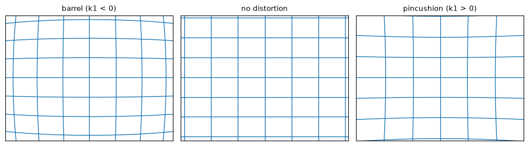The same flat grid through three lenses. Radial distortion grows with distance from the principal point, so straight lines bend most near the image corners.

Rendering synthetic calibration images with known truth

With a real camera you never know the true parameters, so you can't tell how accurate a calibration is. With a synthetic camera you can. The renderer below creates a photo of a checkerboard (9 × 6 inner corners, 25 mm squares, with a white border) as seen by K_true with distortion d_true, from any pose.

It uses inverse mapping, like warpPerspective: for each pixel, convert to distorted normalized coordinates, undistort them by fixed-point iteration, cast the ray \((x, y, 1)\) from the camera center, intersect it with the board plane \(Z_w = 0\), and look up the color of the square it hits. Each pixel averages four sub-pixel samples to anti-alias the edges, and a little Gaussian noise is added.

COLS, ROWS, SQ = 9, 6, 25.0                                       # inner corners and square size (mm)
board = np.array([[i * SQ, j * SQ, 0.0] for j in range(ROWS) for i in range(COLS)])

def undistort_normalized(xd, yd, d, iters=8):
    """Invert the distortion model by fixed-point iteration."""
    k1, k2, p1, p2, k3 = d
    x, y = xd.copy(), yd.copy()
    for _ in range(iters):
        r2 = x * x + y * y
        radial = 1 + k1 * r2 + k2 * r2 ** 2 + k3 * r2 ** 3
        dx = 2 * p1 * x * y + p2 * (r2 + 2 * x * x)
        dy = p1 * (r2 + 2 * y * y) + 2 * p2 * x * y
        x, y = (xd - dx) / radial, (yd - dy) / radial
    return x, y

def render_board(rvec, tvec, K, d, rng, noise=2.0):
    R, t = rodrigues(rvec), np.asarray(tvec, float)
    u, v = np.meshgrid(np.arange(W, dtype=float), np.arange(H, dtype=float))
    acc = np.zeros((H, W))
    for du, dv in [(-0.25, -0.25), (0.25, -0.25), (-0.25, 0.25), (0.25, 0.25)]:
        yd = (v + dv - K[1, 2]) / K[1, 1]
        xd = (u + du - K[0, 2]) / K[0, 0]
        x, y = undistort_normalized(xd, yd, d)
        ray = np.stack([x, y, np.ones_like(x)], axis=-1)
        s = (R[:, 2] @ t) / (ray @ R[:, 2])                       # ray length to the plane Z_w = 0
        Xw = (s[..., None] * ray - t) @ R                         # back to world coordinates: R^T (X_c - t)
        X, Y = Xw[..., 0], Xw[..., 1]
        dark = (np.floor(X / SQ + 1) + np.floor(Y / SQ + 1)) % 2 == 0
        on_squares = (X > -SQ) & (X < COLS * SQ) & (Y > -SQ) & (Y < ROWS * SQ)
        on_border = (X > -2 * SQ) & (X < (COLS + 1) * SQ) & (Y > -2 * SQ) & (Y < (ROWS + 1) * SQ)
        acc += np.where(on_squares, np.where(dark, 0.1, 0.95), np.where(on_border, 0.95, 0.45))
    img = acc / 4 * 255 + rng.normal(0, noise, (H, W))
    return np.clip(img, 0, 255).astype(np.uint8)

def random_pose(rng, z_range=(420, 650)):
    """A pose that keeps the board in view, tilted up to about 30 degrees."""
    rvec = np.array([rng.uniform(-0.5, 0.5), rng.uniform(-0.5, 0.5), rng.uniform(-0.3, 0.3)])
    center = np.array([(COLS - 1) * SQ / 2, (ROWS - 1) * SQ / 2, 0.0])
    where = np.array([rng.uniform(-60, 60), rng.uniform(-40, 40), rng.uniform(*z_range)])
    return rvec, where - rodrigues(rvec) @ center                # board center lands at `where`

rng = np.random.default_rng(0)
poses = [random_pose(rng) for _ in range(14)]
views = [render_board(r, t, K_true, d_true, rng) for r, t in poses]
print(f"rendered {len(views)} views of shape {views[0].shape}, dtype {views[0].dtype}")

rendered 14 views of shape (480, 640), dtype uint8

Calibrating with OpenCV and measuring the error

Now treat the renders as if they came from an unknown camera: detect the corners, refine them, and calibrate. Because you know the true corner positions (from project), you can also measure the corner detector's own accuracy.

criteria = (cv2.TERM_CRITERIA_EPS + cv2.TERM_CRITERIA_MAX_ITER, 30, 0.01)
obj_points, img_points, corner_err = [], [], []
for (rvec, tvec), img in zip(poses, views):
    found, corners = cv2.findChessboardCorners(img, (COLS, ROWS))
    if not found:
        continue
    corners = cv2.cornerSubPix(img, corners, (5, 5), (-1, -1), criteria)
    truth = project(board, rvec, tvec, K_true, d_true)
    corner_err.append(np.linalg.norm(corners.reshape(-1, 2) - truth, axis=1))
    obj_points.append(board.astype(np.float32))
    img_points.append(corners)
corner_err = np.concatenate(corner_err)
print(f"boards found: {len(img_points)}/{len(views)}; corner error vs truth: "
      f"mean {corner_err.mean():.3f} px, max {corner_err.max():.3f} px")

rms, K_est, d_est, rvecs, tvecs = cv2.calibrateCamera(obj_points, img_points, (W, H), None, None,
                                                      flags=cv2.CALIB_FIX_K3)
d_est = d_est.ravel()
print(f"RMS reprojection error: {rms:.3f} px\n")
print(f"{'param':6s} {'true':>9s} {'estimated':>10s} {'error':>8s}")
for name, tv, ev in [("fx", K_true[0, 0], K_est[0, 0]), ("fy", K_true[1, 1], K_est[1, 1]),
                     ("cx", K_true[0, 2], K_est[0, 2]), ("cy", K_true[1, 2], K_est[1, 2])]:
    print(f"{name:6s} {tv:9.2f} {ev:10.2f} {ev - tv:8.2f}")
for name, tv, ev in zip(["k1", "k2", "p1", "p2"], d_true, d_est):
    print(f"{name:6s} {tv:9.4f} {ev:10.4f} {ev - tv:8.4f}")

boards found: 14/14; corner error vs truth: mean 0.113 px, max 0.403 px
RMS reprojection error: 0.132 px

param       true  estimated    error
fx        820.00     818.61    -1.39
fy        810.00     808.68    -1.32
cx        322.00     322.33     0.33
cy        238.00     237.89    -0.11
k1       -0.2800    -0.2833  -0.0033
k2        0.0900     0.1131   0.0231
p1        0.0012     0.0010  -0.0002
p2       -0.0008    -0.0011  -0.0003

The focal lengths are within 0.2% and the principal point within half a pixel, from 14 views with corners accurate to about a tenth of a pixel. \(k_1\) is within about 1%. \(k_2\) is off by about 25% in relative terms, but that's less alarming than it sounds: \(k_2\) multiplies \(r^4\), which is small except in the extreme corners, so a range of \(k_2\) values produce nearly identical pixel positions. What matters is whether the model predicts pixels correctly, which you can check directly by comparing the true and estimated distortion across the image:

uu, vv = np.meshgrid(np.linspace(0, W, 33), np.linspace(0, H, 25))
pix = np.column_stack([uu.ravel(), vv.ravel()]).astype(np.float32)
und_true = cv2.undistortPoints(pix.reshape(-1, 1, 2), K_true, d_true, P=K_true).reshape(-1, 2)
und_est = cv2.undistortPoints(pix.reshape(-1, 1, 2), K_est, d_est, P=K_true).reshape(-1, 2)
diff = np.linalg.norm(und_true - und_est, axis=1)
print(f"undistorted pixel disagreement (true vs estimated model): mean {diff.mean():.2f} px, max {diff.max():.2f} px")

undistorted pixel disagreement (true vs estimated model): mean 0.50 px, max 0.91 px

Across the image, undistorting with the estimated model instead of the true one moves points by about half a pixel on average, and up to about a pixel in the extreme corners, where no board corner was ever observed and the model is extrapolating. That's the practical meaning of "covering the frame" in the workflow box: the model is only constrained where you've shown it data.

fig, axes = plt.subplots(1, 4, figsize=(10, 2.2))
for ax, i in zip(axes, [0, 3, 7, 11]):
    vis = cv2.cvtColor(views[i], cv2.COLOR_GRAY2RGB)
    cv2.drawChessboardCorners(vis, (COLS, ROWS), img_points[i], True)
    ax.imshow(vis); ax.axis("off"); ax.set_title(f"view {i}", fontsize=9)
plt.tight_layout(); plt.show()

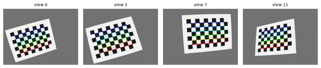Synthetic calibration images rendered through the distorted camera model, with the detected inner corners drawn in order.

Common mistake: counting squares instead of inner corners

findChessboardCorners(img, (9, 6)) looks for 9 × 6 inner corners, where four squares meet, which is a board of 10 × 7 squares. Passing the number of squares makes the detector fail silently (found is False). Also, objectPoints must list the 3D corners in the same order as the detector returns them: row by row, starting from the first corner it finds. For an asymmetric board (odd × even inner corners, like 9 × 6) that order is unambiguous; for a symmetric one it can flip between views.

Zhang's closed-form initialization from scratch

OpenCV hides the initialization inside calibrateCamera. Here's the closed-form step on its own. To isolate it from distortion, which the closed form ignores, generate distortion-free projections of the board in the same poses, with 0.1-pixel noise. Then estimate one homography per view (with the DLT from the previous chapter), build the linear system for \(\boldsymbol{\omega}\), solve it by SVD, and factor \(\boldsymbol{\omega}\) to get \(\mathbf{K}\).

def dlt_homography(src, dst):
    """Normalized DLT (from the Matching and RANSAC chapter), dst ~ H src."""
    def norm(P):
        c = P.mean(0); s = np.sqrt(2) / np.linalg.norm(P - c, axis=1).mean()
        T = np.array([[s, 0, -s * c[0]], [0, s, -s * c[1]], [0, 0, 1]])
        return T, (np.column_stack([P, np.ones(len(P))]) @ T.T)[:, :2]
    T1, a = norm(src); T2, b = norm(dst)
    A = []
    for (x, y), (u, v) in zip(a, b):
        A += [[x, y, 1, 0, 0, 0, -u * x, -u * y, -u], [0, 0, 0, x, y, 1, -v * x, -v * y, -v]]
    Hn = np.linalg.svd(np.array(A))[2][-1].reshape(3, 3)
    Hm = np.linalg.inv(T2) @ Hn @ T1
    return Hm / Hm[2, 2]

def v_ij(Hm, i, j):
    """Row of the linear system for omega = K^-T K^-1, from columns i and j of H."""
    hi, hj = Hm[:, i], Hm[:, j]
    return np.array([hi[0] * hj[0], hi[0] * hj[1] + hi[1] * hj[0], hi[1] * hj[1],
                     hi[2] * hj[0] + hi[0] * hj[2], hi[2] * hj[1] + hi[1] * hj[2], hi[2] * hj[2]])

def zhang_intrinsics(homographies):
    V = []
    for Hm in homographies:
        V.append(v_ij(Hm, 0, 1))                       # h1^T w h2 = 0
        V.append(v_ij(Hm, 0, 0) - v_ij(Hm, 1, 1))      # h1^T w h1 - h2^T w h2 = 0
    b = np.linalg.svd(np.array(V))[2][-1]
    B = np.array([[b[0], b[1], b[3]], [b[1], b[2], b[4]], [b[3], b[4], b[5]]])
    if B[0, 0] < 0:                                    # omega is defined up to sign; make it positive definite
        B = -B
    L = np.linalg.cholesky(B)                          # B = L L^T, with L proportional to K^-T
    K = np.linalg.inv(L.T)
    return K / K[2, 2]

no_dist = np.zeros(5)
Hs = [dlt_homography(board[:, :2], project(board, r, t, K_true, no_dist) + rng.normal(0, 0.1, (len(board), 2)))
      for r, t in poses]
K_zhang = zhang_intrinsics(Hs)
np.set_printoptions(precision=2, suppress=True)
print("Zhang closed form (no distortion, 0.1 px noise):\n", K_zhang)

Hs_dist = [dlt_homography(board[:, :2], c.reshape(-1, 2)) for c in img_points]
print("Closed form on the real (distorted) corners:\n", zhang_intrinsics(Hs_dist))

Zhang closed form (no distortion, 0.1 px noise):
 [[819.37  -0.22 322.27]
 [  0.   809.34 237.53]
 [  0.     0.     1.  ]]
Closed form on the real (distorted) corners:
 [[828.84  -2.44 317.66]
 [  0.   816.72 270.08]
 [  0.     0.     1.  ]]

Without distortion, about twenty lines of linear algebra recover \(\mathbf{K}\) to within a pixel, with a skew that's essentially zero. On the distorted corners the closed form is biased by up to 30 pixels (look at \(c_y\)), because a homography can't represent barrel distortion. That's exactly why OpenCV uses it only to initialize the Levenberg-Marquardt refinement that adds the distortion model.

Undistorting images

With \(\mathbf{K}\) and the distortion coefficients, cv2.undistort removes the distortion from a whole image. The newCameraMatrix argument controls the output's framing, and cv2.getOptimalNewCameraMatrix(K, d, size, alpha) computes one:

• alpha=0 crops so that every output pixel is valid (no black regions), at the cost of losing some of the original field of view at the edges.
• alpha=1 keeps every original pixel, at the cost of black curved borders.

To check that the undistortion actually straightens lines, fit a straight line to each row of detected corners (in the original distorted image, and after undistorting the corner positions with cv2.undistortPoints) and measure the residual.

def row_straightness(pts):
    """RMS distance of each row of corners from its best-fit line, averaged over rows."""
    pts = pts.reshape(ROWS, COLS, 2)
    res = []
    for row in pts:
        c = row - row.mean(0)
        res.append(np.linalg.svd(c, compute_uv=False)[-1] / np.sqrt(len(row)))
    return np.mean(res)

i = int(np.argmax([row_straightness(c) for c in img_points]))       # the most visibly distorted view
raw = img_points[i].reshape(-1, 2)
und = cv2.undistortPoints(img_points[i], K_est, d_est, P=K_est).reshape(-1, 2)
print(f"view {i}: corner rows, RMS deviation from a straight line: distorted {row_straightness(raw):.3f} px, "
      f"undistorted {row_straightness(und):.3f} px")

newK0, roi0 = cv2.getOptimalNewCameraMatrix(K_est, d_est, (W, H), alpha=0)
newK1, roi1 = cv2.getOptimalNewCameraMatrix(K_est, d_est, (W, H), alpha=1)
und0 = cv2.undistort(views[i], K_est, d_est, None, newK0)
und1 = cv2.undistort(views[i], K_est, d_est, None, newK1)
print(f"new focal length: alpha=0 -> {newK0[0, 0]:.1f}, alpha=1 -> {newK1[0, 0]:.1f} (original {K_est[0, 0]:.1f})")

fig, axes = plt.subplots(1, 3, figsize=(10, 2.7))
for ax, im, title in zip(axes, [views[i], und0, und1], ["distorted input", "undistorted, alpha=0", "undistorted, alpha=1"]):
    ax.imshow(im, cmap="gray"); ax.set_title(title, fontsize=10); ax.axis("off")
plt.tight_layout(); plt.show()

view 1: corner rows, RMS deviation from a straight line: distorted 0.435 px, undistorted 0.103 px
new focal length: alpha=0 -> 782.5, alpha=1 -> 761.0 (original 818.6)

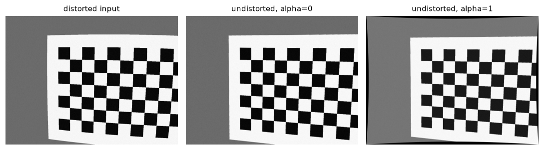Undistortion straightens the board's rows. With alpha=0 the output is cropped to valid pixels; with alpha=1 all source pixels are kept and black borders appear.

In the most distorted view, the rows of corners bow measurably in the raw image and are straight to about the corner detector's noise level after undistortion. Notice also that both new camera matrices have a smaller focal length than the original: to fit the stretched corners of the undistorted image into the same \(640 \times 480\) frame, the output is effectively zoomed out.

Common mistake: undistorting points without P

cv2.undistortPoints(pts, K, d) returns normalized coordinates (\(x_n, y_n\), around \(\pm 0.4\)), not pixels. Pass P=K (or the new camera matrix) to get pixel coordinates back. Mixing the two produces points clustered in the top-left corner and confusing bugs downstream.

For video, compute the undistortion maps once with cv2.initUndistortRectifyMap and apply cv2.remap to every frame. cv2.undistort recomputes the maps on every call.

Pose with PnP and an augmented-reality cube

Render a new view the calibration never saw, detect its corners, and recover the board's pose with cv2.solvePnP, using the estimated intrinsics and distortion. Then compare with the true pose and draw a virtual cube standing on the board.

rng_pose = np.random.default_rng(42)
r_new, t_new = random_pose(rng_pose)
img_new = render_board(r_new, t_new, K_true, d_true, rng_pose)
found, c_new = cv2.findChessboardCorners(img_new, (COLS, ROWS))
c_new = cv2.cornerSubPix(img_new, c_new, (5, 5), (-1, -1), criteria)

ok, r_pnp, t_pnp = cv2.solvePnP(board, c_new, K_est, d_est)
R_err = rodrigues(r_pnp) @ rodrigues(r_new).T
angle_err = np.degrees(np.arccos(np.clip((np.trace(R_err) - 1) / 2, -1, 1)))
cam_true = -rodrigues(r_new).T @ t_new
cam_pnp = -rodrigues(r_pnp).T @ t_pnp.ravel()
print(f"rotation error: {angle_err:.3f} degrees")
print(f"camera center: true {cam_true.round(1)} mm, PnP {cam_pnp.round(1)} mm, "
      f"error {np.linalg.norm(cam_true - cam_pnp):.2f} mm at distance {np.linalg.norm(cam_true):.0f} mm")

# A cube of side 3 squares standing on the board. The camera is on the -Z side of the board,
# so "up" toward the camera is -Z.
s3 = 3 * SQ
base = np.array([[0, 0, 0], [s3, 0, 0], [s3, s3, 0], [0, s3, 0]], float) + [3 * SQ, 1 * SQ, 0]
cube = np.vstack([base, base - [0, 0, s3]])
uv, _ = cv2.projectPoints(cube, r_pnp, t_pnp, K_est, d_est)
uv = uv.reshape(-1, 2).astype(int)

ar = cv2.cvtColor(img_new, cv2.COLOR_GRAY2RGB)
cv2.drawContours(ar, [uv[:4]], -1, (0, 200, 0), -1)                         # floor
for a_, b_ in [(0, 4), (1, 5), (2, 6), (3, 7)]:
    cv2.line(ar, tuple(uv[a_]), tuple(uv[b_]), (30, 90, 255), 3)             # pillars
cv2.drawContours(ar, [uv[4:]], -1, (255, 60, 60), 3)                         # top
cv2.drawFrameAxes(ar, K_est, d_est, r_pnp, t_pnp, 2 * SQ, 3)
plt.figure(figsize=(5.5, 4.2)); plt.imshow(ar); plt.axis("off")
plt.title("PnP pose + projected cube and board axes"); plt.tight_layout(); plt.show()

rotation error: 0.055 degrees
camera center: true [  26.1  -70.5 -627.5] mm, PnP [  26.4  -69.8 -626.6] mm, error 1.21 mm at distance 632 mm

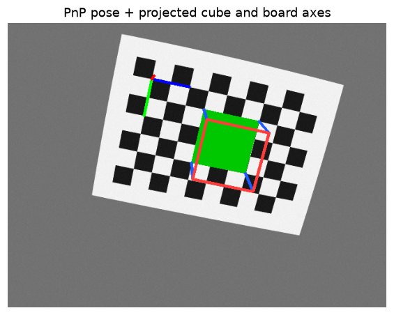The cube's base is locked to the board squares and its vertical edges converge with the correct perspective, because it was projected with the estimated K, distortion, and pose.

The pose is accurate to about a twentieth of a degree, and the camera position to about a millimeter at more than 60 cm (0.2%), using intrinsics estimated from other images. drawFrameAxes draws the board's \(X\), \(Y\), and \(Z\) axes in red, green, and blue in BGR order. This image is RGB, so the colors of \(X\) and \(Z\) swap: the long blue line along the top row of squares is the \(X\) axis, and the short red stub at the origin is \(Z\), foreshortened because it points almost straight away from the camera. That's also why the cube had to be built along \(-Z\) to stand up toward the viewer. It's a small instance of the BGR-versus-RGB trap: OpenCV's drawing functions don't know which order your array is in.

Common mistake: forgetting distortion in PnP or projection

solvePnP(objectPoints, imagePoints, K, dist) interprets the image points as distorted pixels (as detected) and undistorts them internally. If you've already undistorted the image, pass dist=None (or zeros) instead; passing the coefficients again "undistorts" twice. The same applies to projectPoints: it applies distortion, so its output matches the raw image, not an undistorted one.

OpenCV 5 notes

OpenCV 5 split the old C++ calib3d module into calib (calibration), geometry (PnP, homographies, triangulation), and stereo. From Python nothing changes: cv2.calibrateCamera, cv2.solvePnP, cv2.findHomography, and the rest keep their names and signatures. The cv2.fisheye submodule is still there for very wide lenses.

Exercises

Exercise 1: Projection by hand (easy)

A camera has \(f_x = f_y = 800\), \(c_x = 320\), \(c_y = 240\), no distortion, and sits at the world origin looking down the world \(Z\) axis (\(\mathbf{R} = \mathbf{I}\), \(\mathbf{t} = \mathbf{0}\)).

1. Where does the point \((0.5, -0.25, 4)\) meters project?
2. A car that's 1.8 m wide spans 120 pixels. Assuming it's roughly facing the camera, how far away is it?
3. What's the camera's horizontal field of view for a 640-pixel-wide image?

Solution

1. \(u = 800 \cdot 0.5/4 + 320 = 420\), \(v = 800 \cdot (-0.25)/4 + 240 = 190\). The point is right of center and above it (negative \(Y\) is up).
2. Width in pixels \(= f_x \cdot W/Z\), so \(Z = f_x W / w_{\text{px}} = 800 \times 1.8 / 120 = 12\) m.
3. \(2\arctan(320/800) = 2 \times 21.8° = 43.6°\).

K1 = np.array([[800.0, 0, 320], [0, 800, 240], [0, 0, 1]])
print(project(np.array([[0.5, -0.25, 4.0]]), np.zeros(3), np.zeros(3), K1, np.zeros(5)))
print(800 * 1.8 / 120, np.degrees(2 * np.arctan(320 / 800)))

[[420. 190.]]
12.0 43.60281897270362

Exercise 2: Counting degrees of freedom (easy)

How many degrees of freedom do \(\mathbf{K}\) (with skew), \(\mathbf{R}\), \(\mathbf{t}\), and \(\mathbf{P}\) have? Use the counts to explain (a) why one view of a planar board can't determine \(\mathbf{K}\) by itself, and (b) why Zhang's method needs at least three views when the skew is unknown.

Solution

\(\mathbf{K}\): 5 (\(f_x, f_y, s, c_x, c_y\)). \(\mathbf{R}\): 3. \(\mathbf{t}\): 3. \(\mathbf{P}\): \(3 \times 4 = 12\) entries minus 1 for scale = 11 = 5 + 3 + 3.

(a) One view of a plane gives one homography: 8 numbers. The pose of that view uses 6 of them, leaving only 2 constraints on \(\mathbf{K}\), which has 5 unknowns. (b) Each additional view adds 8 numbers but also 6 new pose unknowns, again leaving 2 constraints on the shared \(\mathbf{K}\). Five unknowns need \(\lceil 5/2 \rceil = 3\) views. With zero skew assumed, 4 unknowns need 2 views; with only the focal length unknown, 1 view can be enough.

Exercise 3: A rotating camera induces a homography (medium)

Verify the claim \(\tilde{\mathbf{u}}_2 \sim \mathbf{K}\mathbf{R}\mathbf{K}^{-1}\tilde{\mathbf{u}}_1\). Generate 200 random 3D points at depths from 1 to 50 meters, project them with K_true (no distortion) from a camera at the origin with \(\mathbf{R} = \mathbf{I}\), and again from a camera at the origin rotated by rvec = (0.05, 0.2, 0.02). Compute \(\mathbf{H} = \mathbf{K}\mathbf{R}\mathbf{K}^{-1}\) and the maximum error when mapping the first set of pixels to the second. Then translate the second camera by 0.3 m sideways and fit the best homography with cv2.findHomography (no RANSAC). What happens to the error, and why?

Solution

rng_ex = np.random.default_rng(1)
dirs = rng_ex.uniform([-0.35, -0.25, 1], [0.35, 0.25, 1], size=(200, 3))
X = dirs * rng_ex.uniform(1000, 50000, size=(200, 1))            # mm, depths 1 to 50 m
r2 = np.array([0.05, 0.2, 0.02])
u1 = project(X, np.zeros(3), np.zeros(3), K_true, no_dist)
u2 = project(X, r2, np.zeros(3), K_true, no_dist)
Hrot = K_true @ rodrigues(r2) @ np.linalg.inv(K_true)
mapped = np.column_stack([u1, np.ones(200)]) @ Hrot.T
print(f"pure rotation: max error of K R K^-1 = {np.abs(mapped[:, :2] / mapped[:, 2:] - u2).max():.2e} px")

u2t = project(X, r2, np.array([300.0, 0, 0]), K_true, no_dist)     # plus 0.3 m translation
Hfit, _ = cv2.findHomography(u1, u2t, 0)
m2 = np.column_stack([u1, np.ones(200)]) @ Hfit.T
err = np.linalg.norm(m2[:, :2] / m2[:, 2:] - u2t, axis=1)
print(f"rotation + translation: best homography error mean {err.mean():.1f} px, max {err.max():.1f} px")

pure rotation: max error of K R K^-1 = 2.27e-13 px
rotation + translation: best homography error mean 14.3 px, max 185.8 px

For a pure rotation, \(\mathbf{K}\mathbf{R}\mathbf{K}^{-1}\) maps every point exactly, regardless of depth. With a 0.3 m translation, points at different depths shift by different amounts (parallax: a point at 1 m moves \(f \cdot 0.3/1 = 246\) pixels, one at 50 m only about 5), and no single homography can fit both. That's why handheld panoramas show ghosting on nearby objects, and why you should rotate the camera about its optical center (with a panoramic head, for example).

Exercise 4: Bad calibration data (medium)

Calibrate again using only views where the board is nearly fronto-parallel: render 10 views with rvec components drawn from \(\pm 0.05\) instead of \(\pm 0.5\), at the same distances. Compare the errors in \(f_x\) and \(c_x\) with the 14-view calibration in the chapter. Explain the result.

Solution

rng_fp = np.random.default_rng(7)
obj_fp, img_fp = [], []
for _ in range(10):
    r, t = random_pose(rng_fp)
    r = r * 0.1                                                    # nearly fronto-parallel
    t = np.array([rng_fp.uniform(-60, 60), rng_fp.uniform(-40, 40), rng_fp.uniform(420, 650)]) \
        - rodrigues(r) @ np.array([(COLS - 1) * SQ / 2, (ROWS - 1) * SQ / 2, 0])
    im = render_board(r, t, K_true, d_true, rng_fp)
    found, c = cv2.findChessboardCorners(im, (COLS, ROWS))
    if found:
        obj_fp.append(board.astype(np.float32))
        img_fp.append(cv2.cornerSubPix(im, c, (5, 5), (-1, -1), criteria))
rms_fp, K_fp, d_fp, _, _ = cv2.calibrateCamera(obj_fp, img_fp, (W, H), None, None, flags=cv2.CALIB_FIX_K3)
print(f"{len(img_fp)} fronto-parallel views: RMS {rms_fp:.3f} px, fx error {K_fp[0, 0] - 820:.1f},"
      f" cx error {K_fp[0, 2] - 322:.1f}")
print(f"14 tilted views:          RMS {rms:.3f} px, fx error {K_est[0, 0] - 820:.1f}, cx error {K_est[0, 2] - 322:.1f}")

10 fronto-parallel views: RMS 0.231 px, fx error 93.6, cx error 3.4
14 tilted views:          RMS 0.132 px, fx error -1.4, cx error 0.3

The RMS reprojection error is still low (0.23 px, which most people would accept as a good calibration), yet the focal length is off by more than 10%. For a board facing the camera, a larger focal length with the board farther away produces almost the same image as a smaller focal length with the board closer: \(f\) and the distance \(t_z\) are nearly interchangeable, since the image size depends on \(f/t_z\). Tilting the board breaks the ambiguity, because the near and far edges then have different depths and the perspective foreshortening depends on \(f\) separately. A low RMS error doesn't mean an accurate calibration: it means the model fits the data, which a wrong model can do when the data doesn't constrain it.

Exercise 5: The projection matrix by DLT, then decomposed (hard)

If the 3D points are not coplanar, you can estimate the full \(3 \times 4\) projection matrix \(\mathbf{P}\) linearly, without knowing \(\mathbf{K}\). Derive the two equations each 3D-2D correspondence gives (in the same way as the homography DLT), implement the DLT for \(\mathbf{P}\) (how many points are needed?), test it on 50 random 3D points projected through K_true, rvec, and tvec from the first code block (no distortion, 0.2 px noise), and recover \(\mathbf{K}\), \(\mathbf{R}\), \(\mathbf{t}\) with cv2.decomposeProjectionMatrix.

Solution

With rows \(\mathbf{p}_1^\top, \mathbf{p}_2^\top, \mathbf{p}_3^\top\) of \(\mathbf{P}\) and \(\tilde{\mathbf{X}}\) the homogeneous 3D point, \(u = \mathbf{p}_1^\top\tilde{\mathbf{X}} / \mathbf{p}_3^\top\tilde{\mathbf{X}}\) gives \(\mathbf{p}_1^\top\tilde{\mathbf{X}} - u\,\mathbf{p}_3^\top\tilde{\mathbf{X}} = 0\), and similarly for \(v\). That's two linear equations in the 12 entries of \(\mathbf{P}\); with 11 degrees of freedom you need at least 6 points (5.5, rounded up), not all on one plane.

def dlt_projection(X, u):
    A = []
    for Xh, (x, y) in zip(np.column_stack([X, np.ones(len(X))]), u):
        A.append(np.r_[Xh, np.zeros(4), -x * Xh])
        A.append(np.r_[np.zeros(4), Xh, -y * Xh])
    return np.linalg.svd(np.array(A))[2][-1].reshape(3, 4)

X50 = pts3d[:50]
u50 = project(X50, rvec, tvec, K_true, no_dist) + np.random.default_rng(3).normal(0, 0.2, (50, 2))
P_est = dlt_projection(X50, u50)
P_est *= np.sign(np.linalg.det(P_est[:, :3]))      # SVD returns P up to sign; choose det(KR) > 0
K_d, R_d, C_h = cv2.decomposeProjectionMatrix(P_est)[:3]
K_d = K_d / K_d[2, 2]
C = (C_h[:3] / C_h[3]).ravel()
print("K from P:\n", K_d)
print("rotation error (deg):",
      np.degrees(np.linalg.norm(cv2.Rodrigues(R_d @ rodrigues(rvec).T)[0])).round(3))
print("camera center:", C.round(2), " true:", (-rodrigues(rvec).T @ tvec).round(2))

K from P:
 [[823.5   -0.11 321.01]
 [  0.   814.56 234.08]
 [  0.     0.     1.  ]]
rotation error (deg): 0.364
camera center: [  56.78 -197.74 -543.28]  true: [  56.41 -197.42 -539.84]

decomposeProjectionMatrix performs an RQ decomposition of the left \(3 \times 3\) block of \(\mathbf{P}\) (upper-triangular \(\mathbf{K}\) times orthogonal \(\mathbf{R}\)) and returns the camera center in homogeneous coordinates. The recovered intrinsics are within a few pixels and the pose within a fraction of a degree. This is how cameras were calibrated with 3D calibration rigs before Zhang's planar method; pixel coordinates in the hundreds make normalization (as in the homography DLT) advisable for real data.

Check yourself

1. Write the full projection from a world point to a pixel, naming each matrix and what it contains.

   Answer

   \(\lambda(u, v, 1)^\top = \mathbf{K}[\mathbf{R} \mid \mathbf{t}](X, Y, Z, 1)^\top\). \(\mathbf{R}, \mathbf{t}\) (extrinsics) move the point into camera coordinates; division by \(Z\) gives normalized coordinates (where distortion is applied); \(\mathbf{K}\) (intrinsics: \(f_x, f_y, c_x, c_y\), skew) converts to pixels.

2. What does the vector \(\mathbf{t}\) returned by solvePnP represent? How do you get the camera's position in the object's frame?

   Answer

   \(\mathbf{t}\) is the object (world) origin expressed in camera coordinates. The camera center in object coordinates is \(\mathbf{C} = -\mathbf{R}^\top\mathbf{t}\).

3. Why can't a single image determine the depth of a point, and what are three ways to get it?

   Answer

   All points on a ray through the camera center project to the same pixel, so depth is lost. You can recover it from a known object size (similar triangles), a second view (stereo or motion, with triangulation), or a known surface (for example, a point on a calibrated ground plane), or with an active sensor.

4. What do \(k_1 < 0\) and \(k_1 > 0\) look like, and why is distortion applied to normalized coordinates?

   Answer

   \(k_1 < 0\) is barrel distortion (edges pulled inward, straight lines bowing outward); \(k_1 > 0\) is pincushion. Applying it in normalized coordinates makes the coefficients independent of the image resolution and focal length in pixels, so they describe the lens itself.

5. Why are tilted views of the board essential for calibration?

   Answer

   With fronto-parallel views, the focal length and the board's distance are nearly interchangeable (image size depends on \(f/Z\)), so \(f\) is poorly constrained. Tilted views put parts of the board at different depths, and the resulting foreshortening constrains \(f\) separately.

6. A calibration reports an RMS reprojection error of 0.1 px. Does that mean the parameters are accurate?

   Answer

   Not necessarily. It means the model fits the detected corners well. If the views don't constrain some parameters (no tilts, corners never near the image edges, too many distortion terms), the fit can be excellent while the parameters are wrong. Check the parameter uncertainties (calibrateCameraExtended returns standard deviations), the coverage of the frame, and ideally the error on held-out views.

7. Why does cv2.undistort with alpha=1 produce black borders, and what changes in the new camera matrix?

   Answer

   Undistorting barrel distortion stretches the image outward, so keeping all source pixels inside the same frame requires zooming out (a smaller new focal length). The regions of the output that map outside the original image have no data and are black. With alpha=0, the new matrix zooms in just enough to crop them away.

Key takeaways

• The pinhole model: \(\lambda\tilde{\mathbf{u}} = \mathbf{K}[\mathbf{R} \mid \mathbf{t}]\tilde{\mathbf{X}}\). \(\mathbf{K}\) holds the intrinsics (\(f_x, f_y, c_x, c_y\)), \(\mathbf{R}, \mathbf{t}\) the pose, and \(\mathbf{P} = \mathbf{K}[\mathbf{R} \mid \mathbf{t}]\) has 11 degrees of freedom.
• \(\mathbf{t}\) is the world origin in camera coordinates; the camera center is \(-\mathbf{R}^\top\mathbf{t}\). OpenCV represents rotations as Rodrigues vectors.
• A plane maps to the image by \(\mathbf{H} = \mathbf{K}[\mathbf{r}_1\;\mathbf{r}_2\;\mathbf{t}]\); a rotating camera by \(\mathbf{H} = \mathbf{K}\mathbf{R}\mathbf{K}^{-1}\).
• Lens distortion (radial \(k_1, k_2, k_3\) and tangential \(p_1, p_2\)) acts on normalized coordinates. OpenCV's order is (k1, k2, p1, p2, k3).
• Zhang's calibration: per-view homographies give linear constraints on \(\mathbf{K}^{-\top}\mathbf{K}^{-1}\), then Levenberg-Marquardt refines everything, including distortion, on reprojection error. Tilted views covering the whole frame matter more than a low RMS.
• PnP recovers an object's pose from 3D-2D correspondences with a calibrated camera, which is the basis of marker-based AR.

Further reading

• Z. Zhang, "A Flexible New Technique for Camera Calibration," IEEE Transactions on Pattern Analysis and Machine Intelligence, 22(11), 2000.
• R. Hartley and A. Zisserman, Multiple View Geometry in Computer Vision, 2nd ed., Cambridge University Press, 2004, chapters 6–7 (camera models and computing \(\mathbf{P}\)) and 8.8 (calibration from the image of the absolute conic).
• V. Lepetit, F. Moreno-Noguer, and P. Fua, "EPnP: An Accurate O(n) Solution to the PnP Problem," International Journal of Computer Vision, 81(2), 2009.
• OpenCV documentation, "Camera Calibration" tutorial and the camera model description in the calibration module reference, at docs.opencv.org.

Next

One calibrated camera can tell you directions but not depths. Two can. Continue with Stereo and multi-view geometry, where you'll derive the epipolar constraint, estimate the fundamental matrix, triangulate points, and compute depth maps.