Level 2 capstone solution: panorama and stereo depth

Level 2 · Capstone solution · Back to the capstone brief

This is one complete solution. Yours doesn't need to match it line for line: different thresholds, a different reference view, or multi-band instead of feathered blending are all fine, as long as you measure against the ground truth and can explain your numbers. The same code is in the repository as two standalone scripts, scripts/capstones/level-2/part_a_panorama.py and scripts/capstones/level-2/part_b_stereo_depth.py. Run either with python <script>.py; each prints its metrics and writes its result images to the current directory.

Part A: a panorama from three views

Geometry helpers

These are the from-scratch tools from Matching and RANSAC: applying a homography, Hartley normalization, the normalized DLT, the RANSAC iteration formula, and adaptive RANSAC with a final refit on all inliers. Every random choice goes through a seeded generator.

import time

import cv2
import numpy as np
from skimage import data


def apply_h(H, pts):
    """Map (N, 2) points through a 3x3 homography."""
    q = np.column_stack([pts, np.ones(len(pts))]) @ H.T
    with np.errstate(divide="ignore", invalid="ignore"):      # degenerate RANSAC samples can give w = 0
        return q[:, :2] / q[:, 2:3]


def translation(tx, ty):
    return np.array([[1, 0, tx], [0, 1, ty], [0, 0, 1.0]])


def normalize_points(P):
    c = P.mean(axis=0)
    s = np.sqrt(2) / np.mean(np.linalg.norm(P - c, axis=1))
    T = np.array([[s, 0, -s * c[0]], [0, s, -s * c[1]], [0, 0, 1]])
    return T, apply_h(T, P)


def dlt_homography(src, dst):
    """Normalized DLT: H with dst ~ H src, from n >= 4 correspondences."""
    T1, a = normalize_points(src)
    T2, b = normalize_points(dst)
    A = []
    for (x, y), (u, v) in zip(a, b):
        A.append([x, y, 1, 0, 0, 0, -u * x, -u * y, -u])
        A.append([0, 0, 0, x, y, 1, -v * x, -v * y, -v])
    H = np.linalg.svd(np.asarray(A))[2][-1].reshape(3, 3)
    H = np.linalg.inv(T2) @ H @ T1
    return H / H[2, 2]


def ransac_iterations(w, s=4, p=0.999):
    w = min(max(w, 1e-6), 1 - 1e-12)
    return int(np.ceil(np.log(1 - p) / np.log(1 - w ** s)))


def ransac_homography(src, dst, thresh=2.0, p=0.999, max_iters=5000, rng=None):
    """Adaptive RANSAC with the 4-point DLT, then a refit on all inliers."""
    rng = rng or np.random.default_rng(0)
    n = len(src)
    best = np.zeros(n, bool)
    N, i = max_iters, 0
    while i < min(N, max_iters):
        idx = rng.choice(n, 4, replace=False)
        i += 1
        H = dlt_homography(src[idx], dst[idx])
        if not np.all(np.isfinite(H)):
            continue
        inl = np.linalg.norm(apply_h(H, src) - dst, axis=1) < thresh
        if inl.sum() > best.sum():
            best = inl
            N = ransac_iterations(inl.mean(), 4, p)
    H = dlt_homography(src[best], dst[best])
    inl = np.linalg.norm(apply_h(H, src) - dst, axis=1) < thresh
    return H, inl, i

The three views and their true homographies

The views are what a camera with focal length 600 px, rotating about its center, would see of the scene in skimage's rocket image: yaw angles of −10°, 0°, and +10°, with a little pitch and roll, and a 300 × 427 sensor. Treating the original photo as the image of a camera \(\mathbf{K}_s\) looking straight ahead, view \(i\) is the scene warped by \(\mathbf{H}_i = \mathbf{K}_v\mathbf{R}_i\mathbf{K}_s^{-1}\), so the true homography from view \(i\) to the middle view is \(\mathbf{H}_1\mathbf{H}_i^{-1} = \mathbf{K}_v\mathbf{R}_1\mathbf{R}_i^\top\mathbf{K}_v^{-1}\). Each view also gets its own exposure gain (0.88, 1.0, 1.15) and a little sensor noise. Using a physically consistent rotating camera (rather than arbitrary warps) matters for the comparison with cv2.Stitcher, whose camera model assumes exactly this.

F_SCENE = 600.0                       # focal length (px) of the camera that "took" the original photo
VIEW_W, VIEW_H = 300, 427             # each view is a narrower camera at the same center
YAW_PITCH_ROLL = [(-10.0, 2.0, 1.0), (0.0, 0.0, 0.0), (10.0, -2.0, -1.5)]   # degrees


def rotation(yaw, pitch, roll):
    """Rotation of the virtual camera: yaw about y (down), pitch about x, roll about z."""
    y, p, r = np.radians([yaw, pitch, roll])
    Ry = np.array([[np.cos(y), 0, np.sin(y)], [0, 1, 0], [-np.sin(y), 0, np.cos(y)]])
    Rx = np.array([[1, 0, 0], [0, np.cos(p), -np.sin(p)], [0, np.sin(p), np.cos(p)]])
    Rz = np.array([[np.cos(r), -np.sin(r), 0], [np.sin(r), np.cos(r), 0], [0, 0, 1]])
    return Rz @ Rx @ Ry


def make_views(seed=0):
    """Three overlapping views from a camera rotating about its center, with different exposures.

    The original photo is treated as the image of a camera with focal length F_SCENE. View i is what
    a camera at the same center, rotated by R_i, with focal length F_SCENE and a 300 x 427 sensor
    would see: H_i = K_view R_i K_scene^-1 maps scene pixels to view pixels.
    """
    scene = data.rocket()                                    # RGB, 427 x 640
    sh, sw = scene.shape[:2]
    K_scene = np.array([[F_SCENE, 0, sw / 2], [0, F_SCENE, sh / 2], [0, 0, 1]])
    K_view = np.array([[F_SCENE, 0, VIEW_W / 2], [0, F_SCENE, VIEW_H / 2], [0, 0, 1]])
    gains = [0.88, 1.0, 1.15]
    rng = np.random.default_rng(seed)
    views, scene_to_view = [], []
    for (yaw, pitch, roll), g in zip(YAW_PITCH_ROLL, gains):
        H = K_view @ rotation(yaw, pitch, roll) @ np.linalg.inv(K_scene)
        img = cv2.warpPerspective(scene, H, (VIEW_W, VIEW_H)).astype(np.float32)
        valid = cv2.warpPerspective(np.full((sh, sw), 255, np.uint8), H, (VIEW_W, VIEW_H),
                                    flags=cv2.INTER_NEAREST)
        img = np.clip(img * g + rng.normal(0, 2.0, img.shape), 0, 255)
        img[valid == 0] = 0
        views.append((img.astype(np.uint8), valid))
        scene_to_view.append(H)
    to_scene = [np.linalg.inv(H) for H in scene_to_view]     # view i pixel -> scene pixel
    ref = 1
    H_true = [scene_to_view[ref] @ to_scene[i] for i in range(3)]   # view i -> view 1
    H_true = [H / H[2, 2] for H in H_true]
    return scene, views, H_true, to_scene

scene, views, H_true, to_scene = make_views()
import matplotlib.pyplot as plt
fig, axes = plt.subplots(1, 4, figsize=(10, 3.2), gridspec_kw={"width_ratios": [640 / 427, 300 / 427, 300 / 427, 300 / 427]})
axes[0].imshow(scene); axes[0].set_title("original scene", fontsize=9)
for ax, (img, _), (yaw, _, _) in zip(axes[1:], views, YAW_PITCH_ROLL):
    ax.imshow(img); ax.set_title(f"view, yaw {yaw:+.0f}°", fontsize=9)
for ax in axes: ax.axis("off")
plt.tight_layout(); plt.show()
print("true homography view 0 -> view 1:\n", np.round(H_true[0], 4))

true homography view 0 -> view 1:
 [[ 9.046000e-01  1.700000e-03  1.058357e+02]
 [-7.590000e-02  9.473000e-01  3.115270e+01]
 [-3.000000e-04 -1.000000e-04  1.000000e+00]]

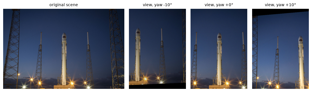The three views overlap by roughly half their width, differ in exposure, and are related by rotations, so straight lines tilt slightly differently in each.

Matching and RANSAC, measured against the truth

For each outer view: SIFT, the ratio test at 0.75, then RANSAC with a 2-pixel threshold. The error metric maps a dense 40 × 40 grid of view points through the estimated and the true homography and measures the distance between the results, both over the part of the view that overlaps the middle view and over the whole view (where the estimate has to extrapolate). cv2.findHomography with RANSAC on the same matches is the reference.

def match_and_estimate(view_src, view_dst, ratio=0.75, seed=0):
    sift = cv2.SIFT_create()
    g1 = cv2.cvtColor(view_src, cv2.COLOR_RGB2GRAY)
    g2 = cv2.cvtColor(view_dst, cv2.COLOR_RGB2GRAY)
    k1, d1 = sift.detectAndCompute(g1, None)
    k2, d2 = sift.detectAndCompute(g2, None)
    pairs = cv2.BFMatcher(cv2.NORM_L2).knnMatch(d1, d2, k=2)
    good = [m for m, n in (p for p in pairs if len(p) == 2) if m.distance < ratio * n.distance]
    src = np.float32([k1[m.queryIdx].pt for m in good])
    dst = np.float32([k2[m.trainIdx].pt for m in good])
    H, inl, iters = ransac_homography(src, dst, thresh=2.0, rng=np.random.default_rng(seed))
    return H, src, dst, inl, iters


def reprojection_error(H_est, H_gt, w, h, mask_fn=None):
    """Mean and max distance between H_est and H_gt applied to a dense grid over a w x h view."""
    grid = np.stack(np.meshgrid(np.linspace(0, w - 1, 40), np.linspace(0, h - 1, 40)), -1).reshape(-1, 2)
    if mask_fn is not None:
        grid = grid[mask_fn(grid)]
    err = np.linalg.norm(apply_h(H_est, grid) - apply_h(H_gt, grid), axis=1)
    return err.mean(), err.max()

H_est = [None, np.eye(3), None]
h, w = views[0][0].shape[:2]
for i in (0, 2):
    H, src, dst, inl, iters = match_and_estimate(views[i][0], views[1][0], seed=i)
    H_est[i] = H
    in_ref = lambda g, i=i: np.all((apply_h(H_true[i], g) >= 0) & (apply_h(H_true[i], g) < [w, h]), axis=1)
    e_ov, e_all = reprojection_error(H, H_true[i], w, h, in_ref), reprojection_error(H, H_true[i], w, h)
    H_cv, _ = cv2.findHomography(src, dst, cv2.RANSAC, 2.0)
    e_cv = reprojection_error(H_cv, H_true[i], w, h, in_ref)
    print(f"view {i} -> view 1: {len(src)} matches, {inl.sum()} inliers ({inl.mean():.0%}), {iters} RANSAC iterations")
    print(f"   ours: overlap mean {e_ov[0]:.2f} px (max {e_ov[1]:.2f}); whole view mean {e_all[0]:.2f} px (max {e_all[1]:.2f})")
    print(f"   cv2.findHomography (RANSAC): overlap mean {e_cv[0]:.2f} px (max {e_cv[1]:.2f})")

view 0 -> view 1: 92 matches, 78 inliers (85%), 10 RANSAC iterations
   ours: overlap mean 0.04 px (max 0.09); whole view mean 0.05 px (max 0.13)
   cv2.findHomography (RANSAC): overlap mean 0.04 px (max 0.10)
view 2 -> view 1: 73 matches, 57 inliers (78%), 16 RANSAC iterations
   ours: overlap mean 0.21 px (max 1.08); whole view mean 0.36 px (max 2.03)
   cv2.findHomography (RANSAC): overlap mean 0.21 px (max 1.08)

Both homographies are accurate to a fraction of a pixel in the overlap and agree with OpenCV's. The adaptive loop stops after a dozen or so iterations, because the inlier ratios are high (the formula needs only tens of samples at these ratios for 99.9% confidence). The view 2 estimate is a little worse than view 0's and degrades more when extrapolated across the whole view, which is consistent with having fewer inliers.

Compositing: canvas, gain compensation, and feathering

The middle view is the reference, so the outer views are warped by their estimated homographies into its frame, shifted by a translation so the canvas starts at \((0, 0)\). The validity masks (eroded by one pixel to drop interpolated border pixels) keep each view's black corners out of the blend. One gain per outer view is estimated by least squares over its overlap with the reference, \(g = \sum I_i I_{\text{ref}} / \sum I_i^2\), and feathering weights each view by its distance transform.

To measure the result against the truth, the panorama is warped back into the original scene's coordinates (through the middle view's known scene mapping) and compared with the original photo, pixel by pixel, wherever the panorama has content.

def gain_compensate(views_w, masks):
    """One gain per image, relative to the reference (index 1), from the overlap with it."""
    gains = [1.0, 1.0, 1.0]
    for i in (0, 2):
        ov = (masks[i] > 0) & (masks[1] > 0)
        a, b = views_w[i][ov], views_w[1][ov]
        gains[i] = float((a * b).sum() / (a * a).sum())
    return gains


def composite(views, homographies, compensate=True):
    corners = []
    for (img, _), H in zip(views, homographies):
        h, w = img.shape[:2]
        corners.append(apply_h(H, np.float32([[0, 0], [w, 0], [w, h], [0, h]])))
    corners = np.vstack(corners)
    xmin, ymin = np.floor(corners.min(axis=0)).astype(int)
    xmax, ymax = np.ceil(corners.max(axis=0)).astype(int)
    T = translation(-xmin, -ymin)
    size = (xmax - xmin, ymax - ymin)
    warped, masks = [], []
    for (img, valid), H in zip(views, homographies):
        warped.append(cv2.warpPerspective(img, T @ H, size).astype(np.float32))
        m = cv2.warpPerspective(valid, T @ H, size, flags=cv2.INTER_NEAREST)
        masks.append(cv2.erode(m, np.ones((3, 3), np.uint8)))          # drop interpolated border pixels
    gains = gain_compensate(warped, masks) if compensate else [1.0, 1.0, 1.0]
    weights = [cv2.distanceTransform((m > 0).astype(np.uint8), cv2.DIST_L2, 5) for m in masks]
    num = sum(w[..., None] * g * im for w, g, im in zip(weights, gains, warped))
    den = sum(weights)[..., None]
    pano = np.clip(num / np.maximum(den, 1e-6), 0, 255).astype(np.uint8)
    coverage = (den[..., 0] > 0)
    return pano, coverage, T, gains


def scene_fidelity(pano, coverage, T, to_scene_ref, scene):
    """Warp the panorama back into original-scene coordinates and compare with the original."""
    h, w = scene.shape[:2]
    M = to_scene_ref @ np.linalg.inv(T)                      # canvas -> scene
    back = cv2.warpPerspective(pano, M, (w, h)).astype(np.float32)
    cov = cv2.warpPerspective(coverage.astype(np.uint8), M, (w, h), flags=cv2.INTER_NEAREST) > 0
    cov = cv2.erode(cov.astype(np.uint8), np.ones((7, 7), np.uint8)) > 0
    err = np.abs(back - scene.astype(np.float32))[cov]
    mse = np.mean(err ** 2)
    return err.mean(), 10 * np.log10(255 ** 2 / mse), cov.mean()

pano, coverage, T, gains = composite(views, H_est)
pano_raw, _, _, _ = composite(views, H_est, compensate=False)
mae, psnr, cov = scene_fidelity(pano, coverage, T, to_scene[1], scene)
mae_raw, psnr_raw, _ = scene_fidelity(pano_raw, coverage, T, to_scene[1], scene)
print(f"estimated gains: {gains[0]:.3f}, 1, {gains[2]:.3f}   (true relative gains {1 / 0.88:.3f}, 1, {1 / 1.15:.3f})")
print(f"panorama vs original: MAE {mae:.2f} gray levels, PSNR {psnr:.1f} dB over {cov:.0%} of the scene")
print(f"without gain compensation: MAE {mae_raw:.2f}, PSNR {psnr_raw:.1f} dB")

estimated gains: 1.141, 1, 0.873   (true relative gains 1.136, 1, 0.870)
panorama vs original: MAE 2.22 gray levels, PSNR 35.0 dB over 80% of the scene
without gain compensation: MAE 7.02, PSNR 29.1 dB

The estimated gains match the true relative exposures to within half a percent, and compensating them cuts the reconstruction error by about a factor of three. The remaining error (about 2 gray levels on average) is the sensor noise added to the views plus interpolation from warping twice.

Comparison with cv2.Stitcher

t0 = time.perf_counter()
stitcher = cv2.Stitcher_create(cv2.Stitcher_PANORAMA)
status, pano_cv = stitcher.stitch([cv2.cvtColor(v, cv2.COLOR_RGB2BGR) for v, _ in views])
print(f"status {status} (0 = OK), views used {[int(i) for i in stitcher.component()]}, "
      f"time {time.perf_counter() - t0:.2f} s, output {pano_cv.shape[1]}x{pano_cv.shape[0]} (ours {pano.shape[1]}x{pano.shape[0]})")
print("estimated focal lengths:", [round(float(c.focal), 1) for c in stitcher.cameras()], " true: 600")
Rs = [np.asarray(c.R, float) for c in stitcher.cameras()]
for i in (0, 2):
    est = np.degrees(np.linalg.norm(cv2.Rodrigues(Rs[i] @ Rs[1].T)[0]))
    true = np.degrees(np.linalg.norm(cv2.Rodrigues(rotation(*YAW_PITCH_ROLL[i]))[0]))
    print(f"rotation view {i} vs view 1: Stitcher {est:.2f} deg, true {true:.2f} deg")

fig, axes = plt.subplots(1, 2, figsize=(10, 4.4))
axes[0].imshow(pano); axes[0].set_title("ours: RANSAC homographies, gains, feathering", fontsize=9)
axes[1].imshow(cv2.cvtColor(pano_cv, cv2.COLOR_BGR2RGB)); axes[1].set_title("cv2.Stitcher (PANORAMA mode)", fontsize=9)
for ax in axes: ax.axis("off")
plt.tight_layout(); plt.show()

status 0 (0 = OK), views used [0, 1, 2], time 0.37 s, output 518x450 (ours 547x509)
estimated focal lengths: [566.0, 566.6, 565.4]  true: 600
rotation view 0 vs view 1: Stitcher 10.82 deg, true 10.23 deg
rotation view 2 vs view 1: Stitcher 10.92 deg, true 10.33 deg

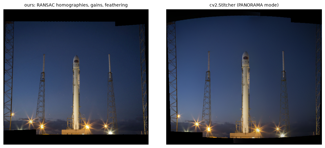Both stitches are seamless. Ours is a planar projection in the middle view's frame; the Stitcher reprojects onto a sphere (note its curved top edge) and uses multi-band blending.

The Stitcher succeeds and looks good, but its output isn't in any frame you can compare pixel by pixel with the truth: it estimates a focal length (here several percent below the true 600 px), rotations (about half a degree too large), and warps onto a sphere. The two errors point in compatible directions: for small pans, a slightly shorter focal length with slightly larger rotations explains the overlaps almost as well, so the two are hard to separate. Two practical observations from building this solution:

• With a 12° pan instead of 10°, the default Stitcher silently dropped one view (component() returned only two indices), because its pairwise confidence fell below panoConfidenceThresh (1.0 by default). Always check component().
• When the views were made with arbitrary per-view perspective warps instead of a consistent rotating camera, lowering the confidence threshold made the Stitcher include all views but produce a hugely distorted panorama thousands of pixels wide: its rotation-only camera model didn't fit the data. A general homography pipeline, like ours, has no such assumption, which is both its strength (it handles planar scenes and arbitrary warps) and its weakness (errors accumulate in long chains and wide pans stretch on a plane).

Part B: depth from the motorcycle stereo pair

Matchers, metrics, and the depth conversion

The left-right consistency check uses a standard trick to get the right view's disparity from the same matcher: flip both images horizontally and swap them, so the right image becomes the "left" one, then flip the result back.

import cv2
import numpy as np
from skimage import data

F_PX, BASELINE_MM, DOFFS = 994.978, 193.001, 31.086
NUM_DISP = 64                     # GT disparities span about 7..60 px


def load():
    left, right, gt = data.stereo_motorcycle()
    valid = np.isfinite(gt)                              # occluded / unknown pixels are inf
    return left, right, np.where(valid, gt, 0).astype(np.float32), valid


def disparity_bm(left, right):
    gl, gr = (cv2.cvtColor(im, cv2.COLOR_RGB2GRAY) for im in (left, right))
    bm = cv2.StereoBM_create(numDisparities=NUM_DISP, blockSize=15)
    return bm.compute(gl, gr).astype(np.float32) / 16.0  # fixed point with 4 fractional bits


def sgbm_matcher(min_disp=0, block=5):
    return cv2.StereoSGBM_create(minDisparity=min_disp, numDisparities=NUM_DISP, blockSize=block,
                                 P1=8 * 3 * block ** 2, P2=32 * 3 * block ** 2,
                                 uniquenessRatio=10, speckleWindowSize=100, speckleRange=2,
                                 disp12MaxDiff=1, mode=cv2.STEREO_SGBM_MODE_SGBM_3WAY)


def disparity_sgbm(left, right):
    return sgbm_matcher().compute(left, right).astype(np.float32) / 16.0


def disparity_sgbm_lr(left, right, tol=1.0):
    """SGBM plus an explicit left-right consistency check.

    The right-view disparity is computed by flipping both images horizontally and swapping them,
    which turns the right view into a "left" view for the same matcher.
    """
    dL = disparity_sgbm(left, right)
    dR = sgbm_matcher().compute(np.ascontiguousarray(right[:, ::-1]),
                                np.ascontiguousarray(left[:, ::-1])).astype(np.float32)[:, ::-1] / 16.0
    h, w = dL.shape
    xs = np.arange(w)[None, :] - np.round(dL).astype(int)
    inside = (xs >= 0) & (dL > 0)
    dR_at = np.take_along_axis(dR, np.clip(xs, 0, w - 1), axis=1)
    keep = inside & (dR_at > 0) & (np.abs(dL - dR_at) <= tol)
    return np.where(keep, dL, 0)


def disparity_metrics(disp, gt, valid):
    has = (disp > 0) & valid
    err = np.abs(disp - gt)[has]
    return {"coverage": has.sum() / valid.sum(), "bad1": np.mean(err > 1), "bad2": np.mean(err > 2),
            "mae": err.mean(), "rmse": np.sqrt(np.mean(err ** 2))}


def to_depth_mm(disp):
    return np.where(disp > 0, F_PX * BASELINE_MM / (disp + DOFFS), np.nan)


def depth_metrics(disp, gt, valid):
    has = (disp > 0) & valid
    Z, Zgt = to_depth_mm(disp)[has], to_depth_mm(gt)[has]
    abs_err = np.abs(Z - Zgt)
    rel = abs_err / Zgt
    return {"median_abs_mm": np.median(abs_err), "mean_abs_mm": abs_err.mean(),
            "abs_rel": rel.mean(), "within_1pct": np.mean(rel < 0.01), "within_5pct": np.mean(rel < 0.05)}


def depth_bands(disp, gt, valid, edges_mm=(2000, 2500, 3000, 3500, 4000, 5100)):
    has = (disp > 0) & valid
    Z, Zgt = to_depth_mm(disp), to_depth_mm(gt)
    rows = []
    for lo, hi in zip(edges_mm[:-1], edges_mm[1:]):
        band = has & (Zgt >= lo) & (Zgt < hi)
        d_err = np.median(np.abs(disp - gt)[band])
        z_err = np.median(np.abs(Z - Zgt)[band])
        zc = (lo + hi) / 2
        predicted = zc ** 2 / (F_PX * BASELINE_MM) * d_err        # Delta Z ~ Z^2 / (f B) * Delta d
        rows.append((lo, hi, int(band.sum()), d_err, z_err, predicted))
    return rows

Disparity and depth accuracy

left, right, gt, valid = load()
print(f"pair {left.shape[1]}x{left.shape[0]}, GT on {valid.mean():.1%} of pixels, "
      f"disparity {gt[valid].min():.1f}..{gt[valid].max():.1f} px, "
      f"depth {np.nanmin(to_depth_mm(gt)[valid]) / 1000:.2f}..{np.nanmax(to_depth_mm(gt)[valid]) / 1000:.2f} m")
results = {"StereoBM": disparity_bm(left, right), "StereoSGBM": disparity_sgbm(left, right),
           "StereoSGBM + LR check": disparity_sgbm_lr(left, right)}
print(f"\n{'method':22s} {'coverage':>8s} {'bad-1':>6s} {'bad-2':>6s} {'MAE':>6s} {'RMSE':>6s}"
      f" | {'med |dZ|':>8s} {'AbsRel':>7s} {'<1%':>5s} {'<5%':>5s}")
for name, disp in results.items():
    m, z = disparity_metrics(disp, gt, valid), depth_metrics(disp, gt, valid)
    print(f"{name:22s} {m['coverage']:8.1%} {m['bad1']:6.1%} {m['bad2']:6.1%} {m['mae']:6.2f} {m['rmse']:6.2f}"
          f" | {z['median_abs_mm']:6.1f}mm {z['abs_rel']:7.2%} {z['within_1pct']:5.0%} {z['within_5pct']:5.0%}")

pair 741x500, GT on 92.7% of pixels, disparity 7.2..59.9 px, depth 2.11..5.02 m

method                 coverage  bad-1  bad-2    MAE   RMSE | med |dZ|  AbsRel   <1%   <5%
StereoBM                  78.4%   8.9%   6.9%   1.21   4.84 |    7.1mm   1.72%   88%   94%
StereoSGBM                87.1%   7.7%   5.9%   1.00   4.10 |    7.4mm   1.47%   89%   95%
StereoSGBM + LR check     81.0%   6.7%   5.0%   0.87   3.70 |    7.1mm   1.26%   90%   96%

The disparity columns use the pixels where each method returns a value (coverage tells you how many that is); "bad-2" is the share of those with an error above 2 px. The depth columns use the same pixels: the median absolute depth error, the mean relative error (AbsRel), and the share within 1% and 5% of the true depth.

• SGBM beats BM on every metric, with 9 points more coverage.
• The left-right check trades 6 points of coverage for a lower bad-pixel rate and RMSE: it removes mostly occluded pixels, whose "matches" are guesses.
• Medians and means tell different stories. The median depth error is about 7 mm for all three, because most pixels are matched to a fraction of a pixel. The mean relative error and the RMSE are dominated by the few gross mismatches, and that's where the methods differ.

Does the error follow the \(Z^2\) law?

print(f"{'depth band (m)':>15s} {'pixels':>7s} {'|dd| px':>8s} {'|dZ| mm':>8s} {'Z^2/(fB)*|dd|':>14s}")
for lo, hi, n, d_err, z_err, pred in depth_bands(results["StereoSGBM"], gt, valid):
    print(f"{lo / 1000:6.1f} - {hi / 1000:4.1f}   {n:7d} {d_err:8.3f} {z_err:8.1f} {pred:14.1f}")

 depth band (m)  pixels  |dd| px  |dZ| mm  Z^2/(fB)*|dd|
   2.0 -  2.5    121852    0.170      4.8            4.5
   2.5 -  3.0     52855    0.173      6.3            6.8
   3.0 -  3.5     12755    0.232     12.9           12.8
   3.5 -  4.0     68175    0.178     12.8           13.0
   4.0 -  5.1     43502    0.232     23.7           25.1

The median disparity error is roughly constant across depth (about 0.17–0.23 px), while the median depth error grows from about 5 mm at 2 m to about 24 mm at 4–5 m. The prediction \(\Delta Z \approx Z^2\Delta d/(fB)\), using each band's own median disparity error and center depth, matches the measured depth error to within a millimeter or two in every band. Strictly, with the principal-point offset, \(Z = fB/(d + d_{\text{offs}})\), so \(|\partial Z/\partial d| = Z^2/(fB)\) still holds exactly.

Z_sgbm, Z_gt = to_depth_mm(results["StereoSGBM"]), to_depth_mm(np.where(valid, gt, 0))
rel_err = np.abs(Z_sgbm - Z_gt) / Z_gt
fig, axes = plt.subplots(1, 4, figsize=(10, 2.3))
axes[0].imshow(left); axes[0].set_title("left image", fontsize=9)
for ax, Z, t in [(axes[1], Z_gt, "GT depth"), (axes[2], Z_sgbm, "SGBM depth")]:
    im = ax.imshow(Z / 1000, cmap="turbo", vmin=2, vmax=5); ax.set_title(t + " (m)", fontsize=9)
im3 = axes[3].imshow(rel_err * 100, cmap="magma", vmin=0, vmax=5); axes[3].set_title("relative error (%)", fontsize=9)
fig.colorbar(im, ax=axes[2], fraction=0.035); fig.colorbar(im3, ax=axes[3], fraction=0.035)
for ax in axes: ax.axis("off")
plt.tight_layout(); plt.show()

Depth is accurate on most surfaces. The largest relative errors sit at object boundaries (foreground fattening), in occluded regions next to them, and on dark, low-texture areas.

Acceptance checklist, checked

Criterion	Result
Own RANSAC + DLT for every homography, seeded	Yes: ransac_homography with np.random.default_rng(seed)
Reprojection error vs the true homographies, in the overlap	About 0.04 px (view 0) and 0.2 px (view 2), mean
Agrees with cv2.findHomography	Same error to within a hundredth of a pixel
Seamless panorama with exposure handling	Gains within 0.5% of truth; PSNR about 35 dB against the original
cv2.Stitcher compared, with its failure modes noted	Status, views used, focal length, and rotations reported
Disparity evaluated with coverage and bad-pixel rates	BM, SGBM, and SGBM + LR check
Depth from \(Z = fB/(d + d_{\text{offs}})\) with stated \(f\), \(B\), \(d_{\text{offs}}\)	Median error about 7 mm; 95% of pixels within 5%
Error growth explained	Matches \(Z^2\Delta d/(fB)\) band by band

Where to go further

• Replace feathering with multi-band blending (a Laplacian pyramid per view, blending each level with a mask blurred at that level's scale), and compare seam visibility in a crop of the overlap.
• Pan through more views and chain homographies; measure how the error grows along the chain, then fix it by estimating rotations and one shared focal length (the Stitcher's model) with a small bundle adjustment.
• Add sub-pixel refinement or a weighted median filter to the disparity, and see which depth bands improve.
• Swap SGBM for a learned stereo network in Level 8 and compare on the same metrics.