The Frequency Domain

Level 1 · Chapter 4 · ⏱️ ~65 min read · Prerequisites: Convolution and filtering, Edges and gradients

Every image is a sum of waves. This chapter covers the intuition behind Fourier series, the 2D discrete Fourier transform and the FFT, magnitude and phase (with the famous swap experiment), the convolution theorem verified numerically, low-pass and high-pass filtering, aliasing and the sampling theorem, and Gaussian and Laplacian pyramids with exact reconstruction.

Why it matters

Sam's team built a retail app that let shoppers photograph a fabric and see it on a sofa. To keep uploads small, the app shrank every photo to a quarter of its width by keeping every fourth pixel. Most photos looked fine. Fine pinstripes and woven textures came out as bold, swirling patterns that weren't in the fabric at all, and customers ordered fabric that looked nothing like what they had seen.

The cause was aliasing: detail finer than the new pixel grid can represent doesn't disappear when you subsample, it masquerades as coarser detail that was never there. The fix is one line, blur before you shrink (or use cv2.INTER_AREA), but you can only see why it works, and how much to blur, in the frequency domain.

The same viewpoint explains why the box filter from Chapter 2 makes some fine patterns invert, why large convolutions are computed with the FFT, how image pyramids work, and how to remove a periodic interference pattern with surgical precision. It's also how the JPEG format thinks about images, and it's the lens that later explains why CNNs can be fooled by high-frequency patterns.

Concepts

Fourier series: signals as sums of waves

In 1807 Joseph Fourier claimed that any periodic function can be written as a sum of sines and cosines of different frequencies. A square wave, for example, with period \(2\pi\):

\[ \operatorname{sq}(x) = \frac{4}{\pi}\left(\sin x + \frac{\sin 3x}{3} + \frac{\sin 5x}{5} + \dots\right). \]

The first term captures the overall up-and-down. Each additional term, at a higher frequency and smaller amplitude, sharpens the corners. Sharp features need high frequencies; smooth features need only low ones. That one sentence is most of the intuition you need for images.

Each sinusoid has three numbers: a frequency (how many cycles per unit length), an amplitude (how strong), and a phase (where its peaks are). The amplitudes tell you how much of each frequency the signal contains; the phases tell you where things happen.

For an image, the building blocks are 2D sinusoidal gratings: stripes with a frequency and an orientation, like corduroy at some angle. A grating \(\cos\big(2\pi(u x / W + v y / H)\big)\) has \(u\) cycles across the image width \(W\) and \(v\) cycles down its height \(H\). Its stripes are perpendicular to the direction \((u, v)\), and its wavelength is \(1/\sqrt{(u/W)^2 + (v/H)^2}\) pixels. Large \((u, v)\) means fine stripes; small means coarse.

The 2D discrete Fourier transform

The discrete Fourier transform (DFT) of an \(H \times W\) image \(f(y, x)\) expresses it as a weighted sum of exactly \(H \times W\) gratings:

\[ F(v, u) = \sum_{y=0}^{H-1} \sum_{x=0}^{W-1} f(y, x)\, e^{-2\pi i \left(\frac{v y}{H} + \frac{u x}{W}\right)}, \]

and the inverse DFT rebuilds the image from them:

\[ f(y, x) = \frac{1}{HW} \sum_{v=0}^{H-1} \sum_{u=0}^{W-1} F(v, u)\, e^{2\pi i \left(\frac{v y}{H} + \frac{u x}{W}\right)}. \]

Here \(i = \sqrt{-1}\), and \(e^{i\phi} = \cos\phi + i \sin\phi\) (Euler's formula) packs a cosine and a sine into one complex number. Read the forward transform as a dot product: \(F(v, u)\) measures how much the image correlates with the grating of frequency \((v, u)\). Each \(F(v, u)\) is a complex number, and the forward and inverse transforms are exact inverses: no information is lost.

A few facts you'll use constantly:

• The DC term. \(F(0, 0) = \sum f\), the sum of all pixels (mean times \(HW\)). "DC" comes from direct current: the zero-frequency, constant component.
• Negative frequencies. Frequencies \(u\) above \(W/2\) are equivalent to negative frequencies \(u - W\), because \(e^{-2\pi i u x / W}\) is periodic in \(u\). The highest representable frequency is \(W/2\) cycles across the image, which is 0.5 cycles per pixel: one light pixel, one dark pixel. That's the Nyquist frequency.
• Conjugate symmetry. For a real image, \(F(-v, -u) = \overline{F(v, u)}\) (the complex conjugate). Half the spectrum is redundant, and np.fft.rfft2 exploits this to save time.
• Centering for display. NumPy stores frequency 0 at index 0. np.fft.fftshift moves it to the center so the spectrum is displayed with low frequencies in the middle and high frequencies at the edges.
• Periodicity. The DFT implicitly treats the image as one tile of an infinite, periodic wallpaper. Where the left edge doesn't match the right edge, the wallpaper has a sharp jump, which shows up as a bright horizontal and vertical cross through the center of the spectrum. Multiplying the image by a smooth window (such as a Hann window) that fades to zero at the borders suppresses this spectral leakage.

Magnitude and phase

Each coefficient is complex, so write it in polar form: \(F(v, u) = \lvert F(v, u) \rvert\, e^{i \phi(v, u)}\). The magnitude \(\lvert F \rvert\) is how strong that grating is; the phase \(\phi\) is how far it's shifted. The magnitude spectrum is what people usually plot, on a log scale (\(\log(1 + \lvert F \rvert)\)), because the DC term and low frequencies are thousands of times larger than the rest.

Natural images have a characteristic spectrum: the magnitude falls off roughly as \(1/\text{frequency}\), so most energy is in low frequencies. Strong edges produce streaks perpendicular to them in the spectrum. Periodic patterns (fences, fabric, halftone print) produce isolated bright peaks.

import numpy as np
import cv2
import matplotlib.pyplot as plt
from scipy import ndimage
from skimage import data, color

xs = np.linspace(0, 4 * np.pi, 800)
H = W = 128
yy, xx = np.mgrid[:H, :W]
grating = np.cos(2 * np.pi * (8 * xx / W + 3 * yy / H))       # 8 cycles across, 3 down
G = np.fft.fftshift(np.fft.fft2(grating))
peaks = np.argwhere(np.abs(G) > 0.5 * np.abs(G).max()) - [H // 2, W // 2]
print("grating spectrum peaks at (v, u) offsets from center:", peaks.tolist())

img = data.camera().astype(np.float64)
F = np.fft.fft2(img)
print("DC term / number of pixels:", (F[0, 0].real / img.size).round(3), "| image mean:", img.mean().round(3))
print("conjugate symmetry holds:", np.allclose(F[5, 7], np.conj(F[-5, -7])))

fig, axes = plt.subplots(1, 4, figsize=(10, 2.6))
for n, ls in [(1, ":"), (3, "--"), (25, "-")]:
    partial = 4 / np.pi * sum(np.sin(k * xs) / k for k in range(1, 2 * n, 2))
    axes[0].plot(xs, partial, ls, lw=1, label=f"{n} term{'s' if n > 1 else ''}")
axes[0].legend(fontsize=7); axes[0].set_title("square wave, partial sums", fontsize=9)
axes[1].imshow(grating, cmap="gray"); axes[1].set_title("grating (u=8, v=3)", fontsize=9)
axes[2].imshow(np.log1p(np.abs(G)), cmap="gray"); axes[2].set_title("its spectrum: two dots", fontsize=9)
axes[3].imshow(np.log1p(np.abs(np.fft.fftshift(F))), cmap="gray"); axes[3].set_title("camera: log magnitude", fontsize=9)
for ax in axes[1:]:
    ax.axis("off")
plt.tight_layout()
plt.show()

grating spectrum peaks at (v, u) offsets from center: [[-3, -8], [3, 8]]
DC term / number of pixels: 129.061 | image mean: 129.061
conjugate symmetry holds: True

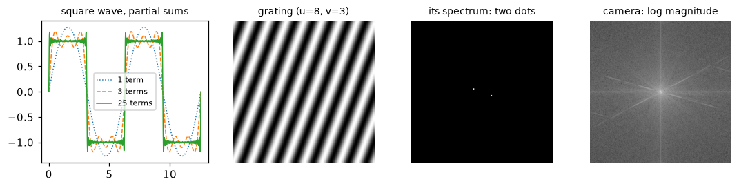
More terms make sharper corners (with a persistent overshoot, the Gibbs phenomenon). A single grating is two dots in the spectrum, at plus and minus its frequency. A natural image has its energy concentrated at the center (low frequencies), plus a cross from the mismatched image borders.

Computing it: the DFT and the FFT

Computed directly from the double sum, each of the \(HW\) coefficients needs \(HW\) multiply-adds: \(O(N^4)\) for an \(N \times N\) image, about \(7 \times 10^{10}\) operations for 512 × 512. Two observations make it fast.

First, the 2D DFT is separable: the exponential factors into \(e^{-2\pi i v y/H}\, e^{-2\pi i u x/W}\), so you can take 1D DFTs of all rows, then of all columns. In matrix form, with the DFT matrix \(\mathbf{W}_N[k, n] = e^{-2\pi i k n / N}\), the transform is \(\mathbf{F} = \mathbf{W}_H\, \mathbf{f}\, \mathbf{W}_W\), two matrix products: \(O(N^3)\).

Second, the fast Fourier transform (FFT; Cooley and Tukey, 1965, though Gauss had the idea around 1805) computes a 1D DFT of length \(N\) in \(O(N \log N)\) instead of \(O(N^2)\). The key step: split the sum into even- and odd-indexed samples. Each half is a DFT of length \(N/2\), and the two halves combine with one multiplication per output (the "twiddle factor" \(e^{-2\pi i k/N}\)). Recursing gives \(\log_2 N\) levels of \(O(N)\) work each. In 2D that's \(O(N^2 \log N)\). The FFT is fastest for sizes with small prime factors; cv2.getOptimalDFTSize and scipy.fft.next_fast_len give good padded sizes.

import time

def dft_matrix(n):
    k = np.arange(n)
    return np.exp(-2j * np.pi * np.outer(k, k) / n)

def dft2_matrix(f):
    """2D DFT as two matrix products (separable), O(N^3)."""
    return dft_matrix(f.shape[0]) @ f @ dft_matrix(f.shape[1])

t0 = time.perf_counter(); F_mat = dft2_matrix(img); t_mat = time.perf_counter() - t0
t0 = time.perf_counter(); F_fft = np.fft.fft2(img); t_fft = time.perf_counter() - t0
print("matrix DFT matches np.fft.fft2:", np.allclose(F_mat, F_fft))
print(f"matrix DFT {t_mat * 1000:.0f} ms | FFT {t_fft * 1000:.1f} ms")
print("inverse recovers the image:", np.allclose(np.fft.ifft2(F_fft).real, img),
      "| max imaginary part:", np.abs(np.fft.ifft2(F_fft).imag).max() < 1e-9)

matrix DFT matches np.fft.fft2: True
matrix DFT 30 ms | FFT 4.2 ms
inverse recovers the image: True | max imaginary part: True

After an inverse FFT of a real image's (possibly filtered) spectrum, the result has tiny imaginary parts from round-off. Take .real, but check that the imaginary part really is tiny: if it isn't, your filter broke conjugate symmetry.

The phase carries the structure

Which matters more for what an image looks like, the magnitude or the phase? Here's the classic experiment (Oppenheim and Lim, 1981): take two images, swap their phases, and invert.

astro = color.rgb2gray(data.astronaut()) * 255                   # also 512 x 512
FA, FB = np.fft.fft2(img), np.fft.fft2(astro)
magA_phaseB = np.fft.ifft2(np.abs(FA) * np.exp(1j * np.angle(FB))).real
magB_phaseA = np.fft.ifft2(np.abs(FB) * np.exp(1j * np.angle(FA))).real

def corr(a, b):
    return np.corrcoef(a.ravel(), b.ravel())[0, 1]
print(f"|camera| + phase(astronaut): corr with camera {corr(magA_phaseB, img):.2f}, with astronaut {corr(magA_phaseB, astro):.2f}")
print(f"|astronaut| + phase(camera): corr with camera {corr(magB_phaseA, img):.2f}, with astronaut {corr(magB_phaseA, astro):.2f}")

fig, axes = plt.subplots(1, 4, figsize=(10, 2.7))
for ax, (im, t) in zip(axes, [(img, "A: camera"), (astro, "B: astronaut"),
                              (magA_phaseB, "magnitude A + phase B"), (magB_phaseA, "magnitude B + phase A")]):
    ax.imshow(im, cmap="gray"); ax.set_title(t, fontsize=9); ax.axis("off")
plt.tight_layout()
plt.show()

|camera| + phase(astronaut): corr with camera 0.11, with astronaut 0.73
|astronaut| + phase(camera): corr with camera 0.73, with astronaut 0.08

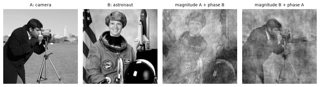
Each hybrid looks like the image whose phase it has. The magnitude only changes the overall texture and contrast.

The phase wins decisively. The reason: edges and lines are places where many frequencies line up in phase (all their peaks coincide at the edge). The phase encodes where things are, and since all natural images have similar \(1/f\) magnitude spectra, the magnitude carries relatively little that distinguishes one image from another. Two consequences: shifting an image changes only its phase (the shift theorem, \(f(x - x_0) \leftrightarrow F(u)\, e^{-2\pi i u x_0 / W}\)), which is the basis of phase-correlation registration (Exercise 6); and a magnitude spectrum alone is a good texture descriptor but a poor shape descriptor.

The convolution theorem

Here's the result that connects this chapter to Chapter 2. Convolution in space is multiplication in frequency:

\[ f * h \;\longleftrightarrow\; F \cdot H. \]

The derivation is short. In 1D with period \(N\), the circular convolution is \(g(x) = \sum_m h(m) f(x - m)\), with indices taken mod \(N\). Take its DFT and substitute \(x' = x - m\):

\[ G(u) = \sum_x \sum_m h(m) f(x - m) e^{-2\pi i u x / N} = \sum_m h(m) e^{-2\pi i u m / N} \sum_{x'} f(x') e^{-2\pi i u x' / N} = H(u)\, F(u). \]

The exponential splits because \(e^{-2\pi i u (x' + m)/N} = e^{-2\pi i u x'/N} e^{-2\pi i u m/N}\), and the shifted sum over \(x'\) still covers one full period. The 2D proof is identical.

What it means:

• Every LSI filter is a frequency-by-frequency gain. \(H(u, v)\), the frequency response (or transfer function), says how much the filter amplifies or attenuates each grating, and \(\angle H\) how much it shifts it. Gratings are the "eigenfunctions" of convolution: a filter can scale and shift a grating but never change its frequency.
• Blur is a low-pass filter. A Gaussian's transform is a Gaussian: \(G_\sigma\) in space has frequency response \(e^{-2\pi^2\sigma^2 f^2}\) (with \(f\) in cycles per pixel), which falls smoothly to zero. Wider in space means narrower in frequency.
• The box filter has negative lobes. Its transform is a sinc-like function, \(\frac{\sin(\pi K f)}{K \sin(\pi f)}\) for width \(K\), which goes negative at some frequencies. A grating at such a frequency comes out inverted (Exercise 3). That's the box's "ripples in frequency" from Chapter 2.
• Derivatives are high-pass. \(\frac{d}{dx} \leftrightarrow 2\pi i u\): differentiation multiplies each frequency by its frequency, which is why it amplifies noise (Chapter 3).
• Big kernels are cheaper in frequency. Direct convolution costs \(O(N^2 K^2)\); via the FFT it's \(O(N^2 \log N)\) no matter how large the kernel.

The DFT's convolution is circular: the kernel wraps around the image's edges, as if the image were periodic. To get ordinary (linear) convolution with zero padding, pad both the image and the kernel to at least \((H + K - 1) \times (W + K - 1)\) before transforming. scipy.signal.fftconvolve does this for you.

from scipy import signal

rng = np.random.default_rng(0)
h = rng.normal(size=(9, 9))                                       # an arbitrary kernel
# Circular convolution via FFT: put the kernel's center at index (0, 0) of an image-sized array
Hpad = np.zeros_like(img)
Hpad[:9, :9] = h
Hpad = np.roll(Hpad, (-4, -4), axis=(0, 1))
via_fft = np.fft.ifft2(np.fft.fft2(img) * np.fft.fft2(Hpad)).real
direct = ndimage.convolve(img, h, mode="wrap")
print("circular: FFT vs direct, max diff:", np.abs(via_fft - direct).max())

lin_fft = signal.fftconvolve(img, h, mode="same")                 # zero-padded linear convolution
lin_direct = ndimage.convolve(img, h, mode="constant")
print("linear (zero padding): fftconvolve vs direct, max diff:", np.abs(lin_fft - lin_direct).max())

for K in [5, 15, 41]:
    k = np.ones((K, K)) / K ** 2
    t0 = time.perf_counter(); ndimage.convolve(img, k, mode="constant"); t_d = time.perf_counter() - t0
    t0 = time.perf_counter(); signal.fftconvolve(img, k, mode="same"); t_f = time.perf_counter() - t0
    print(f"K={K:2d}: direct {t_d * 1000:7.1f} ms | FFT {t_f * 1000:5.1f} ms")

circular: FFT vs direct, max diff: 3.637978807091713e-12
linear (zero padding): fftconvolve vs direct, max diff: 4.092726157978177e-12
K= 5: direct     3.2 ms | FFT   5.8 ms
K=15: direct    31.5 ms | FFT   5.0 ms
K=41: direct   254.8 ms | FFT   5.9 ms

The theorem holds to round-off, both in its circular form and with padding for linear convolution. The FFT route costs the same at every kernel size, so it loses for tiny kernels and wins by a growing margin for large ones. (For separable kernels like the Gaussian, two 1D passes are usually faster still.)

Low-pass and high-pass filtering

With the convolution theorem, you can design filters directly in frequency: build a mask \(H(v, u)\), multiply, invert. Let \(D(v, u)\) be the distance of frequency \((v, u)\) from the center of the shifted spectrum, in cycles per image.

• The ideal low-pass filter keeps every frequency with \(D \le D_0\) and removes the rest. It sounds perfect and isn't: its spatial kernel is a 2D sinc, with ripples that extend far from the center, so every edge in the output gets echoed by faint ringing (the Gibbs phenomenon you saw on the square wave).
• The Gaussian low-pass filter \(H = e^{-D^2 / (2 D_0^2)}\) rolls off smoothly. Its spatial kernel is a Gaussian, so there's no ringing. A frequency-domain Gaussian with standard deviation \(D_0\) cycles per image corresponds to a spatial Gaussian with \(\sigma = \frac{N}{2\pi D_0}\) pixels for an \(N\)-pixel side.
• A high-pass filter is \(1 - H_{\text{low}}\): it keeps edges and fine texture and removes the smooth background. A band-pass filter keeps a ring of frequencies, which isolates detail at one scale (that's what each Laplacian-pyramid level does).

Hh, Ww = img.shape
v = np.fft.fftshift(np.fft.fftfreq(Hh)) * Hh                      # cycles per image, centered
u = np.fft.fftshift(np.fft.fftfreq(Ww)) * Ww
D = np.hypot(*np.meshgrid(v, u, indexing="ij"))
D0 = 30
ideal = (D <= D0).astype(float)
gauss = np.exp(-D ** 2 / (2 * D0 ** 2))

def apply(img, Hmask):
    Fs = np.fft.fftshift(np.fft.fft2(img))
    return np.fft.ifft2(np.fft.ifftshift(Fs * Hmask)).real

low_ideal, low_gauss, high_gauss = apply(img, ideal), apply(img, gauss), apply(img, 1 - gauss)
sigma_spatial = Hh / (2 * np.pi * D0)
spatial = ndimage.gaussian_filter(img, sigma_spatial, mode="wrap", truncate=6)
print(f"frequency Gaussian D0={D0} <-> spatial sigma {sigma_spatial:.3f} px; max diff {np.abs(low_gauss - spatial).max():.4f}")

fig, axes = plt.subplots(1, 4, figsize=(10, 2.7))
crop = (slice(60, 260), slice(180, 380))
for ax, (im, t) in zip(axes, [(img, "original"), (low_ideal, f"ideal low-pass, D0={D0}"),
                              (low_gauss, f"Gaussian low-pass, D0={D0}"), (high_gauss, "Gaussian high-pass")]):
    ax.imshow(im[crop], cmap="gray"); ax.set_title(t, fontsize=9); ax.axis("off")
plt.tight_layout()
plt.show()

frequency Gaussian D0=30 <-> spatial sigma 2.716 px; max diff 0.0000

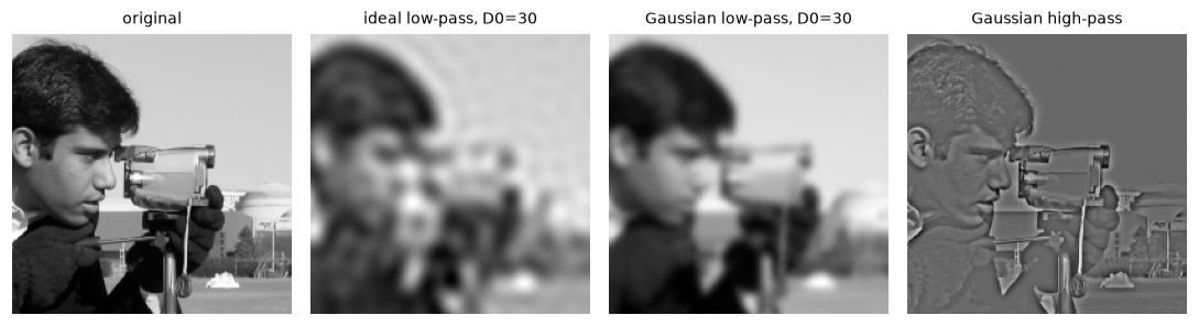
The ideal low-pass echoes every edge with faint ripples. The Gaussian low-pass is clean, and identical to an ordinary spatial Gaussian blur. The high-pass keeps edges and texture on a flat gray background.

Aliasing and the sampling theorem

A digital image is a set of samples of a continuous scene. How fine must the samples be? The Nyquist-Shannon sampling theorem answers: a signal containing no frequencies above \(f_{\max}\) can be reconstructed exactly from samples taken at a rate above \(2 f_{\max}\). Equivalently, a grid with spacing of 1 pixel can represent frequencies only up to 0.5 cycles per pixel, the Nyquist frequency.

What happens to a frequency above Nyquist? It doesn't vanish. Sampled, it produces exactly the same values as some lower frequency, its alias. A frequency \(f\) (in cycles per sample) is indistinguishable from \(f - n\) for any integer \(n\), and since \(\cos\) is even, from \(\lvert f - n \rvert\). So 0.8 cycles per sample looks exactly like 0.2. That's why wagon wheels spin backward in films, why fine fabrics produce moiré patterns, and why Sam's pinstripes turned into swirls.

Downsampling is sampling again. Keeping every \(s\)-th pixel moves the Nyquist limit from 0.5 to \(0.5/s\) cycles per original pixel. Any content between \(0.5/s\) and 0.5 aliases. The cure is to remove it before subsampling with a low-pass filter, called an anti-aliasing filter: you lose fine detail you couldn't have kept anyway, instead of converting it into fake coarse detail. A Gaussian with \(\sigma\) around \(s/2\) is a common rule of thumb (a compromise: it can't cut off perfectly sharply, and a larger \(\sigma\) blurs more than necessary). cv2.resize(..., interpolation=cv2.INTER_AREA) averages over each output pixel's footprint, which is a box prefilter, and skimage.transform.resize(..., anti_aliasing=True) uses a Gaussian.

A zone plate, a pattern whose frequency grows steadily from the center outward, shows aliasing vividly: every frequency is present somewhere, so every alias shows up as a ghost ring.

# 1D first: a frequency of 0.4 cycles/sample, subsampled by 2, becomes 0.8 -> aliases to 0.2
n = np.arange(512)
wave = np.cos(2 * np.pi * 0.4 * n)
sub = wave[::2]
apparent = np.argmax(np.abs(np.fft.rfft(sub))) / sub.size
print(f"after subsampling by 2: apparent frequency {apparent:.3f} cycles/sample (true 0.8 -> alias 0.2)")

N = 512
yy, xx = np.mgrid[-N // 2:N // 2, -N // 2:N // 2]
zone = 0.5 + 0.5 * np.cos(np.pi * (xx ** 2 + yy ** 2) / N)        # local frequency r/N cycles/px
naive = zone[::4, ::4]
prefiltered = ndimage.gaussian_filter(zone, sigma=2.0)[::4, ::4]
area = cv2.resize(zone, (N // 4, N // 4), interpolation=cv2.INTER_AREA)
true_small = np.zeros_like(naive)                                  # what the small image *should* be:
r_small = np.hypot(*np.mgrid[-64:64, -64:64]) * 4                  # the zone plate's content below the new Nyquist
ok = r_small < N / 8                                               # radius where frequency < 0.125 cycles/px
for name, im in [("naive", naive), ("Gaussian prefilter", prefiltered), ("INTER_AREA", area)]:
    print(f"{name:18s} contrast (std) outside the representable zone: {im[~ok].std():.3f}")

fig, axes = plt.subplots(1, 4, figsize=(10, 2.7))
for ax, (im, t) in zip(axes, [(zone, "zone plate 512×512"), (naive, "every 4th pixel"),
                              (prefiltered, "Gaussian σ=2, then subsample"), (area, "cv2.INTER_AREA")]):
    ax.imshow(im, cmap="gray", vmin=0, vmax=1, interpolation="nearest"); ax.set_title(t, fontsize=9); ax.axis("off")
plt.tight_layout()
plt.show()

after subsampling by 2: apparent frequency 0.199 cycles/sample (true 0.8 -> alias 0.2)
naive              contrast (std) outside the representable zone: 0.354
Gaussian prefilter contrast (std) outside the representable zone: 0.016
INTER_AREA         contrast (std) outside the representable zone: 0.062

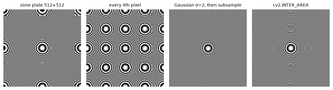
Naive subsampling fills the outer region with ghost rings: frequencies too high for the small grid, aliased to low ones. The Gaussian prefilter turns them into flat gray, the honest answer. The box-like INTER_AREA filter suppresses them only partly. (Even the full-size zone plate aliases in its corners, where its frequency passes 0.5 cycles per pixel.)

Outside the central zone, the small image has no way to represent the true pattern, so the correct output is a flat gray. Naive subsampling instead puts full-contrast fake rings there. The Gaussian prefilter removes almost all of them; INTER_AREA, a box filter, leaves some, because a box's frequency response has those negative lobes and doesn't fall to zero. Aliasing in a camera happens at capture: that's why many cameras have an optical low-pass filter in front of the sensor, and why some high-resolution cameras that omit it can show moiré on fabrics.

Image pyramids

Many tasks need an image at several scales: detecting objects of unknown size, coarse-to-fine motion estimation, multi-scale blending. An image pyramid is a stack of copies at decreasing resolution.

The Gaussian pyramid is built by repeatedly blurring and subsampling by 2:

\[ G_0 = f, \qquad G_{i+1} = \operatorname{down}\big(w * G_i\big), \]

where \(w\) is a small low-pass kernel and \(\operatorname{down}\) keeps every second row and column. The standard kernel, from Burt and Adelson (1983), is the 5-tap binomial \(\frac{1}{16}[1, 4, 6, 4, 1]\) applied separably, a cheap approximation of a Gaussian with \(\sigma \approx 1\). It's the anti-aliasing filter for a factor of 2. Each level has a quarter of the pixels of the one before, so the whole pyramid costs only \(1 + \frac14 + \frac1{16} + \dots = \frac43\) of the original's storage.

Each Gaussian level is a low-pass version of the previous one. What did each blur remove? Upsample the next level back to the current size, \(\operatorname{up}(G_{i+1})\) (insert zeros between samples, then filter with \(4w\) to interpolate), and subtract. That difference is a band-pass image, the detail between two scales. These differences form the Laplacian pyramid:

\[ L_i = G_i - \operatorname{up}(G_{i+1}), \qquad L_n = G_n \text{ (the top level, a tiny blurry image)}. \]

(The name comes from the fact that a difference of two Gaussian-blurred images approximates a Laplacian of Gaussian, Chapter 3.) The Laplacian pyramid is exactly invertible, by construction: start from the top and work down,

\[ G_i = L_i + \operatorname{up}(G_{i+1}). \]

No property of the filter is needed; each step just adds back what was subtracted. Why bother? Because the \(L_i\) are mostly near zero (detail is sparse), they compress well, and they let you manipulate each scale separately. Pyramid blending, the classic application, blends two images with a soft seam at coarse levels and a sharp seam at fine levels, which hides the transition (Exercise 5). Pyramids also underlie SIFT's scale space, optical flow, and the feature pyramid networks in Level 4.

w5 = np.array([1, 4, 6, 4, 1]) / 16.0

def blur5(f, gain=1.0):
    k = w5 * gain
    out = ndimage.correlate1d(f, k, axis=0, mode="mirror")           # mirror = BORDER_REFLECT_101
    return ndimage.correlate1d(out, k, axis=1, mode="mirror")

def pyr_down(f):
    return blur5(f)[::2, ::2]

def pyr_up(f, shape):
    up = np.zeros(shape)
    up[::2, ::2] = f                                                  # zeros between samples
    return blur5(up, gain=2.0)                                        # 2 per axis = 4 in 2D

g1 = pyr_down(img)
print("pyr_down matches cv2.pyrDown:", np.allclose(g1, cv2.pyrDown(img)))
up_ours, up_cv = pyr_up(g1, img.shape), cv2.pyrUp(g1, dstsize=img.shape[::-1])
print("pyr_up matches cv2.pyrUp:", np.allclose(up_ours, up_cv))

levels = 4
gauss_pyr = [img]
for _ in range(levels):
    gauss_pyr.append(pyr_down(gauss_pyr[-1]))
lap_pyr = [gauss_pyr[i] - pyr_up(gauss_pyr[i + 1], gauss_pyr[i].shape) for i in range(levels)] + [gauss_pyr[-1]]

recon = lap_pyr[-1]
for L in reversed(lap_pyr[:-1]):
    recon = L + pyr_up(recon, L.shape)
print("reconstruction max error:", np.abs(recon - img).max())
print("shapes:", [g.shape for g in gauss_pyr])
print("fraction of L0 coefficients with |value| < 5:", np.mean(np.abs(lap_pyr[0]) < 5).round(3))

fig, axes = plt.subplots(2, 5, figsize=(10, 4.4))
for i in range(5):
    axes[0, i].imshow(gauss_pyr[i], cmap="gray"); axes[0, i].set_title(f"G{i} {gauss_pyr[i].shape[0]}²", fontsize=9)
    lim = np.percentile(np.abs(lap_pyr[i]), 99) if i < 4 else None
    axes[1, i].imshow(lap_pyr[i], cmap="gray", vmin=-lim if lim else None, vmax=lim)
    axes[1, i].set_title(f"L{i}", fontsize=9)
for ax in axes.ravel():
    ax.axis("off")
plt.tight_layout()
plt.show()

pyr_down matches cv2.pyrDown: True
pyr_up matches cv2.pyrUp: True
reconstruction max error: 0.0
shapes: [(512, 512), (256, 256), (128, 128), (64, 64), (32, 32)]
fraction of L0 coefficients with |value| < 5: 0.699

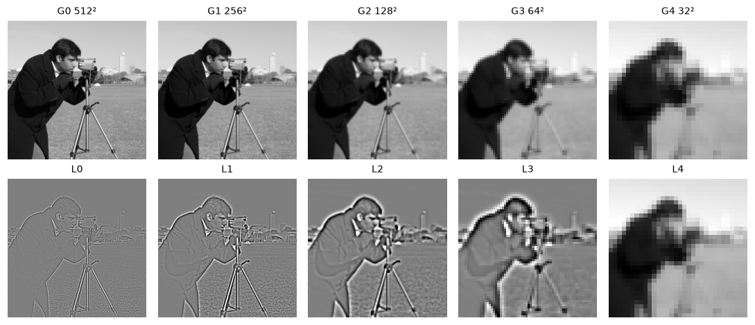
Each Gaussian level is a blurrier, smaller copy. Each Laplacian level holds the detail of one octave of scale: fine texture and edges in L0, the man's outline in L2 and L3.

The from-scratch pyramid matches OpenCV's pyrDown and pyrUp exactly. Reconstruction is exact, and about 70% of the finest Laplacian level is nearly zero (within ±5 levels), which is why pyramids (and their cousins, wavelets) compress so well.

In practice

Removing periodic noise with a notch filter

Periodic interference, from electrical hum in a video signal, a scanner's mechanism, or a halftone print screen, is spread over every pixel in space but concentrated in a few points in frequency. Remove those points and the interference vanishes, with almost no effect on the rest of the image. A notch filter does this: a mask that is 1 everywhere except for small (preferably smooth) holes at the interference peaks and their symmetric twins.

def psnr(a, b):
    return 10 * np.log10(255 ** 2 / np.mean((a - b) ** 2))

yy, xx = np.mgrid[:Hh, :Ww]
noisy = img + 40 * np.cos(2 * np.pi * (30 * xx / Ww + 50 * yy / Hh))

Fs = np.fft.fftshift(np.fft.fft2(noisy))
logmag = np.log1p(np.abs(Fs))
search = logmag.copy()
search[D < 15] = 0                                                # ignore the natural low frequencies
pk = np.argwhere(search >= np.sort(search.ravel())[-2])           # the two strongest peaks
print("peaks found at (v, u) offsets:", (pk - [Hh // 2, Ww // 2]).tolist())

notch = np.ones_like(D)
vv, uu = np.mgrid[:Hh, :Ww]
for (pv, pu) in pk:
    notch *= 1 - np.exp(-((vv - pv) ** 2 + (uu - pu) ** 2) / (2 * 3.0 ** 2))   # smooth Gaussian hole
cleaned = np.fft.ifft2(np.fft.ifftshift(Fs * notch)).real
print(f"PSNR noisy {psnr(noisy, img):.1f} dB | notch-filtered {psnr(cleaned, img):.1f} dB")

fig, axes = plt.subplots(1, 3, figsize=(10, 3.3))
axes[0].imshow(np.clip(noisy, 0, 255), cmap="gray"); axes[0].set_title("periodic interference", fontsize=9)
axes[1].imshow(logmag, cmap="gray"); axes[1].set_title("spectrum: two bright peaks", fontsize=9)
for (pv, pu) in pk:
    axes[1].add_patch(plt.Circle((pu, pv), 12, fill=False, color="tab:red"))
axes[2].imshow(cleaned, cmap="gray"); axes[2].set_title("after the notch filter", fontsize=9)
for ax in axes:
    ax.axis("off")
plt.tight_layout()
plt.show()

peaks found at (v, u) offsets: [[-50, -30], [50, 30]]
PSNR noisy 19.1 dB | notch-filtered 53.6 dB

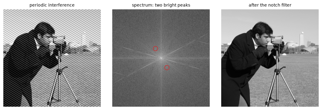
The stripes cover every pixel, but in the spectrum they're just two points. Notching them out raises the PSNR by more than 30 dB.

No spatial filter could do this: any blur strong enough to remove the stripes would destroy the image. In the frequency domain, signal and interference barely overlap, so they separate cleanly.

When to work in the frequency domain

Task	Frequency-domain tool	Library
Convolution with a large kernel (roughly > 15 × 15)	FFT convolution	scipy.signal.fftconvolve, cv2.filter2D (switches automatically)
Remove periodic noise	Notch filter	np.fft.fft2 + mask
Find a translation between two images	Phase correlation	cv2.phaseCorrelate, skimage.registration.phase_cross_correlation
Analyze texture or detect periodicity	Magnitude spectrum	np.fft.fft2, np.abs, np.fft.fftshift
Downsample without aliasing	Low-pass, then subsample	cv2.resize(..., INTER_AREA), cv2.pyrDown, skimage.transform.resize(anti_aliasing=True)
Multi-scale analysis, blending	Gaussian and Laplacian pyramids	cv2.pyrDown, cv2.pyrUp, skimage.transform.pyramid_gaussian
Deblurring with a known blur	Wiener filter	skimage.restoration.wiener

Common mistake: circular wrap-around

Multiplying FFTs gives circular convolution: content near the right edge leaks into the left edge. For linear convolution, pad the image and kernel to at least \((H + K - 1) \times (W + K - 1)\), or use scipy.signal.fftconvolve, which pads for you.

Common mistake: plotting the spectrum without log or shift

plt.imshow(np.abs(np.fft.fft2(img))) shows a black image with four bright corners: the DC term dominates, and zero frequency sits at the corners. Use np.log1p(np.abs(np.fft.fftshift(F))).

Common mistake: subsampling without a prefilter

img[::4, ::4] and cv2.resize(..., interpolation=cv2.INTER_NEAREST) (or INTER_LINEAR for large reductions) alias. For shrinking, use INTER_AREA, a pyramid, or blur first. This applies to data loaders too: a training pipeline that shrinks images with nearest-neighbor creates moiré that a model may learn to rely on.

Exercises

Exercise 1: A DFT by hand (easy)

Compute the 1D DFT of \(f = [1, 2, 3, 4]\) by hand, using \(F(u) = \sum_{x=0}^{3} f(x)\, e^{-2\pi i u x / 4}\) and the fact that \(e^{-2\pi i / 4} = -i\). Check the DC term and conjugate symmetry, then verify with np.fft.fft.

Solution

With \(\omega = -i\): \(F(u) = \sum_x f(x)(-i)^{ux}\).

• \(F(0) = 1 + 2 + 3 + 4 = 10\) (the DC term, the sum).
• \(F(1) = 1 + 2(-i) + 3(-1) + 4(i) = -2 + 2i\).
• \(F(2) = 1 + 2(-1) + 3(1) + 4(-1) = -2\).
• \(F(3) = 1 + 2(i) + 3(-1) + 4(-i) = -2 - 2i\).

\(F(3) = \overline{F(1)}\), since frequency 3 is frequency \(-1\): conjugate symmetry for a real signal.

print(np.fft.fft([1, 2, 3, 4]))

[10.+0.j -2.+2.j -2.+0.j -2.-2.j]

Exercise 2: Shifts change only the phase (medium)

Prove the shift theorem in 1D: if \(g(x) = f(x - x_0)\) (circularly), then \(G(u) = F(u)\, e^{-2\pi i u x_0 / N}\). Then verify in 2D: shift the camera image with np.roll by (37, -50) and show that the magnitude spectrum is unchanged while the phase is not.

Solution

\(G(u) = \sum_x f(x - x_0) e^{-2\pi i u x / N}\). Substitute \(x' = x - x_0\): \(G(u) = \sum_{x'} f(x') e^{-2\pi i u (x' + x_0)/N} = e^{-2\pi i u x_0 / N} F(u)\). The factor has magnitude 1, so \(\lvert G \rvert = \lvert F \rvert\), and the phase changes by \(-2\pi u x_0 / N\), a linear ramp in \(u\).

shifted = np.roll(img, (37, -50), axis=(0, 1))
F1, F2 = np.fft.fft2(img), np.fft.fft2(shifted)
print("magnitudes equal:", np.allclose(np.abs(F1), np.abs(F2)))
print("phases equal:", np.allclose(np.angle(F1), np.angle(F2)))
v, u = 3, 5
predicted = F1[v, u] * np.exp(-2j * np.pi * (v * 37 / 512 + u * (-50) / 512))
print("shift theorem at (3, 5):", np.isclose(F2[v, u], predicted))

magnitudes equal: True
phases equal: False
shift theorem at (3, 5): True

This is why the magnitude spectrum is a translation-invariant descriptor, and why phase correlation can measure translations (Exercise 6).

Exercise 3: The box filter inverts some patterns (medium)

The 1D frequency response of a centered box of width \(K\) is \(H(f) = \frac{\sin(\pi K f)}{K \sin(\pi f)}\) for \(f\) in cycles per pixel. For \(K = 5\), compute \(H(0.3)\). Before running code, predict what a 5-wide box blur does to a grating \(\cos(2\pi \cdot 0.3\, x)\). Then check: filter the grating and compare it with the original.

Solution

\(H(0.3) = \frac{\sin(1.5\pi)}{5 \sin(0.3\pi)} = \frac{-1}{5 \times 0.809} \approx -0.247\). Negative: the grating comes out at a quarter of its amplitude, inverted (peaks become troughs).

x = np.arange(400)
grat = np.cos(2 * np.pi * 0.3 * x)
boxed = ndimage.uniform_filter1d(grat, 5, mode="wrap")
inner = slice(20, -20)
print("predicted H(0.3):", round(np.sin(1.5 * np.pi) / (5 * np.sin(0.3 * np.pi)), 3))
print("measured ratio:", round(np.dot(boxed[inner], grat[inner]) / np.dot(grat[inner], grat[inner]), 3))
print("Gaussian (sigma=1.2) response at 0.3:", round(np.exp(-2 * np.pi ** 2 * 1.2 ** 2 * 0.3 ** 2), 3))

predicted H(0.3): -0.247
measured ratio: -0.247
Gaussian (sigma=1.2) response at 0.3: 0.077

A Gaussian of similar width attenuates the grating more and never inverts it, because its frequency response is positive everywhere. This is the concrete reason the Gaussian is preferred over the box for anti-aliasing and smoothing.

Exercise 4: Predict the alias (medium)

A 1D grating at 0.35 cycles per pixel is subsampled by keeping every third sample. Without running code, predict the frequency you'll see in the subsampled signal, in cycles per new sample. Then verify with an FFT, and show that blurring with a Gaussian of \(\sigma = 1.5\) before subsampling suppresses it.

Solution

In units of the new sample spacing, the frequency is \(0.35 \times 3 = 1.05\) cycles per new sample, far above the new Nyquist of 0.5. Subtracting the nearest integer: \(1.05 - 1 = 0.05\). You'll see a slow wave at 0.05 cycles per new sample, a period of 20 new samples, which was not in the original at all.

n = np.arange(3000)
g = np.cos(2 * np.pi * 0.35 * n)
for name, sig in [("naive", g), ("Gaussian sigma=1.5 first", ndimage.gaussian_filter1d(g, 1.5))]:
    s = sig[::3]
    spec = np.abs(np.fft.rfft(s)) / s.size
    k = np.argmax(spec[1:]) + 1
    print(f"{name:25s} peak at {k / s.size:.3f} cycles/sample, amplitude {2 * spec[k]:.3f}")

naive                     peak at 0.050 cycles/sample, amplitude 1.000
Gaussian sigma=1.5 first  peak at 0.050 cycles/sample, amplitude 0.005

Naive subsampling produces a full-strength fake wave. The prefilter shrinks it to half a percent, matching the Gaussian's theoretical response at 0.35 cycles per pixel, \(e^{-2\pi^2 \cdot 2.25 \cdot 0.1225} \approx 0.004\). The alias is still there, just too weak to matter.

Exercise 5: Pyramid blending (hard)

Blend the left half of the camera image with the right half of the grayscale astronaut. Compare (a) a hard seam, (b) a seam feathered by a Gaussian-blurred mask, and (c) Laplacian pyramid blending: build Laplacian pyramids of both images and a Gaussian pyramid of the binary mask, combine each level as \(L^{\text{out}}_i = M_i L^A_i + (1 - M_i) L^B_i\), and reconstruct. Score each result two ways: the seam step, the largest jump between neighboring columns of a blurred version (\(\sigma = 4\)) near the seam relative to the median jump elsewhere; and the detail kept, the standard deviation of the high-pass detail (\(f - G_{1.5} * f\)) in a 40-pixel band around the seam, relative to the average of the two inputs in that band.

Solution

def lap_pyramid(f, levels):
    gp = [f]
    for _ in range(levels):
        gp.append(pyr_down(gp[-1]))
    return [gp[i] - pyr_up(gp[i + 1], gp[i].shape) for i in range(levels)] + [gp[-1]]

def reconstruct(lp):
    out = lp[-1]
    for L in reversed(lp[:-1]):
        out = L + pyr_up(out, L.shape)
    return out

mask = np.zeros_like(img); mask[:, :256] = 1.0
hard = mask * img + (1 - mask) * astro
soft_mask = ndimage.gaussian_filter(mask, 20)
feathered = soft_mask * img + (1 - soft_mask) * astro

levels = 5
LA, LB = lap_pyramid(img, levels), lap_pyramid(astro, levels)
gm = [mask]
for _ in range(levels):
    gm.append(pyr_down(gm[-1]))
blended = reconstruct([m * a + (1 - m) * b for m, a, b in zip(gm, LA, LB)])

def highpass(x):
    return x - ndimage.gaussian_filter(x, 1.5)
band = slice(236, 276)
ref = 0.5 * (highpass(img)[:, band].std() + highpass(astro)[:, band].std())
for name, im in [("hard seam", hard), ("feathered", feathered), ("pyramid blend", blended)]:
    d = np.abs(np.diff(ndimage.gaussian_filter(im, 4), axis=1)).mean(axis=0)
    step = d[248:264].max() / np.median(d)
    detail = highpass(im)[:, band].std() / ref
    print(f"{name:14s} seam step {step:.2f} | detail kept {detail:.2f}")

hard seam      seam step 4.40 | detail kept 1.05
feathered      seam step 2.05 | detail kept 0.74
pyramid blend  seam step 2.53 | detail kept 0.94

The hard seam is a sharp vertical edge, a jump several times larger than anywhere else. Feathering with one wide blur hides the jump best, but it creates a ghostly double-exposure band about 40 pixels wide where both images' fine details are averaged together, and averaging two unrelated textures washes them out: only about three quarters of the detail survives. Pyramid blending nearly matches feathering's seam score while keeping almost all the detail. It uses a wide transition for the coarse levels (the mask is blurry at the top of its Gaussian pyramid) and a narrow one for the fine levels, so the low frequencies merge smoothly while fine details switch over quickly without ghosting. This is Burt and Adelson's 1983 "multiresolution spline", still used in panorama stitching (Level 2).

Exercise 6: Registration by phase correlation (hard)

Two photos differ by an unknown translation. Using the shift theorem, the normalized cross-power spectrum \(R = \frac{F_1 \overline{F_2}}{\lvert F_1 \overline{F_2} \rvert}\) is a pure phase ramp, and its inverse FFT is a single spike at the shift. Implement it, and recover the shift between img and np.roll(img, (23, -41), axis=(0, 1)) with added Gaussian noise (σ = 20). Compare with cv2.phaseCorrelate.

Solution

If \(f_2(x) = f_1(x - x_0)\), then \(F_2 = F_1 e^{-2\pi i u x_0/N}\), so \(F_1\overline{F_2} = \lvert F_1 \rvert^2 e^{2\pi i u x_0/N}\), and after normalizing to unit magnitude, \(R = e^{2\pi i u x_0/N}\). Its inverse DFT is an impulse at \(-x_0\) (mod \(N\)), so compute it with \(F_2 \overline{F_1}\) instead to get the spike at \(+x_0\).

rng = np.random.default_rng(3)
moved = np.roll(img, (23, -41), axis=(0, 1)) + rng.normal(0, 20, img.shape)
F1, F2 = np.fft.fft2(img), np.fft.fft2(moved)
cross = F2 * np.conj(F1)
r = np.fft.ifft2(cross / (np.abs(cross) + 1e-12)).real
dy, dx = np.unravel_index(np.argmax(r), r.shape)
dy, dx = (dy + 256) % 512 - 256, (dx + 256) % 512 - 256            # wrap to signed shifts
print("ours (row, col):", (int(dy), int(dx)), "| peak height:", r.max().round(3))
(cx, cy), response = cv2.phaseCorrelate(img, moved)
print("cv2.phaseCorrelate (x, y):", (round(cx, 2), round(cy, 2)))

ours (row, col): (23, -41) | peak height: 0.37
cv2.phaseCorrelate (x, y): (-41.02, 23.03)

Both recover the shift exactly, despite heavy noise. Note OpenCV's (x, y) order versus NumPy's (row, col): the classic convention trap. OpenCV also refines the peak to sub-pixel precision, and accepts an optional window (for example, one from cv2.createHanningWindow) to suppress the edge effects of the periodic DFT; it doesn't apply one unless you pass it. Phase correlation is fast (two FFTs) and robust to brightness changes, because normalization discards the magnitude. It's used for video stabilization, microscope drift correction, and as the first step of image stitching when the motion is mostly translation.

Check yourself

1. What does a single coefficient \(F(v, u)\) of the 2D DFT represent?

   Answer

   How strongly (magnitude) and with what shift (phase) the grating with \(u\) cycles across and \(v\) cycles down is present in the image. It's the dot product of the image with that complex sinusoid.

2. Why does the camera image's spectrum have a bright cross through its center?

   Answer

   The DFT treats the image as periodic. The left and right (and top and bottom) edges don't match, so the periodic extension has sharp vertical and horizontal jumps, which put energy along the horizontal and vertical frequency axes. A window function suppresses it.

3. In the magnitude/phase swap experiment, which image does the hybrid resemble, and why?

   Answer

   The one whose phase it has. Phase encodes where structures are (edges are where frequencies align in phase), while the magnitude spectra of natural images are all similar, roughly \(1/f\).

4. State the convolution theorem and one practical consequence.

   Answer

   Convolution in space equals multiplication in frequency: \(f * h \leftrightarrow FH\). Consequences: large convolutions are cheaper via the FFT; any LSI filter is a per-frequency gain; blur is low-pass, derivatives are high-pass.

5. Why does an ideal low-pass filter ring, and how do you avoid it?

   Answer

   Its spatial kernel is a sinc with slowly decaying ripples, which echo every edge. Use a filter with a smooth transition, such as a Gaussian, whose spatial kernel has no ripples.

6. What is aliasing, and how do you prevent it when downsampling by 4?

   Answer

   Frequencies above the new grid's Nyquist limit (\(0.5/4 = 0.125\) cycles per original pixel) fold back and appear as false lower frequencies. Low-pass filter first (Gaussian with \(\sigma\) around 2, a pyramid, or INTER_AREA), then subsample.

7. How is a Laplacian pyramid level computed, and why is the pyramid exactly invertible?

   Answer

   \(L_i = G_i - \operatorname{up}(G_{i+1})\). Reconstruction adds back exactly what was subtracted: \(G_i = L_i + \operatorname{up}(G_{i+1})\), starting from the stored top level. It works for any filter, because nothing is approximated.

8. Why does cv2.phaseCorrelate return (x, y) while your NumPy code finds (row, col)?

   Answer

   OpenCV's geometric functions use \((x, y)\) = (column, row) order, while NumPy indexes arrays as (row, column). Always check which convention a function uses.

Key takeaways

• Every image is a weighted sum of sinusoidal gratings. The DFT finds the weights; the FFT computes them in \(O(N^2 \log N)\). Low frequencies hold smooth content; high frequencies hold edges, texture, and noise.
• Magnitude says how much of each frequency there is; phase says where things are, and it carries most of the visible structure.
• The convolution theorem turns filtering into multiplication: blur is low-pass, derivatives are high-pass, and big kernels are cheaper via the FFT (remember: the DFT's convolution is circular).
• Design filters with smooth transitions (Gaussian) to avoid ringing; notch filters remove periodic noise that no spatial filter could.
• Sampling at spacing 1 can represent frequencies up to 0.5 cycles per pixel. Anything higher aliases into false patterns, so always low-pass before you downsample.
• Gaussian pyramids are blur-and-subsample stacks; Laplacian pyramids store the band-pass differences, reconstruct exactly, and power blending, compression, and multi-scale methods.

Further reading

• Rafael C. Gonzalez and Richard E. Woods, Digital Image Processing, 4th edition, chapter 4 (filtering in the frequency domain). The standard treatment, with many worked examples.
• Peter J. Burt and Edward H. Adelson, "The Laplacian Pyramid as a Compact Image Code", IEEE Transactions on Communications, 1983; and "A Multiresolution Spline with Application to Image Mosaics", ACM Transactions on Graphics, 1983.
• Alan V. Oppenheim and Jae S. Lim, "The Importance of Phase in Signals", Proceedings of the IEEE, 1981.
• Richard Szeliski, Computer Vision: Algorithms and Applications, 2nd edition, sections 3.4–3.5 (Fourier transforms and pyramids), free at szeliski.org/Book.
• NumPy documentation: Discrete Fourier Transform (numpy.fft).

Next

So far every operation treated the image as a grid of intensities. Next you'll treat it as a collection of shapes: Morphology and classical segmentation.