Matching and RANSAC

Level 2 · Chapter 2 · ⏱️ ~75 min read · Prerequisites: Features and keypoints, Geometric transformations (homogeneous coordinates and homographies)

Keypoints and descriptors give you candidate correspondences between two images. This chapter turns them into geometry. You'll compare descriptors with the right distance, speed up matching with approximate nearest neighbors, filter ambiguous matches with the ratio test, and then deal with the matches that are still wrong. RANSAC, derived and built from scratch, finds the model that the correct matches agree on. You'll implement the Direct Linear Transform for homographies, check it against cv2.findHomography, and stitch a panorama with blending.

Why it matters

Sam was building a document-capture feature for an insurance app: photograph a printed claim form, and the app warps it to a clean, flat template so the fields can be read. The pipeline matched ORB features between the photo and the template, then fit a homography with least squares to all the matches.

It worked on Sam's test photos. In production, roughly one capture in ten came out as a wildly distorted, unusable image. The culprit was a handful of wrong matches: the form had a repeated grid of identical checkboxes, and ORB happily matched checkbox 3 in the photo to checkbox 7 in the template. Least squares gives every match a vote, and a few matches that are off by hundreds of pixels dominate the squared error. Five wrong matches out of two hundred were enough to wreck the fit.

Replacing least squares with RANSAC took one argument (cv2.RANSAC in the findHomography call) and the failure rate dropped to almost zero. But Sam's team only trusted it after understanding why it works: how many random samples it needs, what the threshold means, and when it can still fail. That's what this chapter covers.

Concepts

Descriptor distances

Matching starts with a distance between descriptors. Which one depends on the descriptor type:

• Euclidean (L2) distance \(\lVert \mathbf{d}_1 - \mathbf{d}_2 \rVert_2\) for floating-point descriptors such as SIFT. Because SIFT vectors are normalized to unit length, the squared L2 distance is \(2 - 2\,\mathbf{d}_1^\top \mathbf{d}_2\), so ranking by L2 is the same as ranking by cosine similarity.
• Hamming distance for binary descriptors (ORB, BRIEF, BRISK): the number of differing bits, \(\operatorname{popcount}(\mathbf{d}_1 \oplus \mathbf{d}_2)\).
• L1 distance is sometimes used for histogram-like descriptors, and RootSIFT (Arandjelović and Zisserman, 2012) applies an elementwise square root to L1-normalized SIFT vectors so that L2 distance on the result corresponds to the Hellinger kernel on the originals. It's a free, often noticeable improvement for retrieval.

Brute-force and approximate matching

Given \(n_1\) descriptors in image 1 and \(n_2\) in image 2, each of dimension \(d\), brute-force matching computes all \(n_1 n_2\) distances and keeps, for each query, the nearest (or the \(k\) nearest) in the other set. That costs \(O(n_1 n_2 d)\). For two images with a few thousand SIFT features each, that's a few hundred million multiply-adds, which takes milliseconds on a modern CPU. Brute force is exact, simple, and usually the right choice for a pair of images.

When one side is huge (matching a query image against a database of millions of features), you need approximate nearest neighbor (ANN) search, which returns the true nearest neighbor most of the time, much faster.

• k-d trees split the space recursively along coordinate axes. In 128 dimensions an exact k-d tree search degenerates to nearly brute force, but randomized k-d forests with a limited number of leaf checks give good approximate answers (Silpa-Anan and Hartley, 2008).
• Hierarchical k-means trees cluster the descriptors recursively and search the closest clusters first.
• Locality-sensitive hashing (LSH) hashes binary descriptors so that similar ones collide, and only compares within buckets.
• Graph-based indexes such as HNSW (hierarchical navigable small-world graphs) are today's standard in vector databases, including those used for image retrieval with learned embeddings.

FLANN (Fast Library for Approximate Nearest Neighbors, Muja and Lowe, 2009) bundles the first three and picks parameters automatically. OpenCV exposes it as cv2.FlannBasedMatcher. The checks parameter trades speed for accuracy: more leaf checks, more often the exact neighbor.

The ratio test

The nearest neighbor is not always a correct match. Some keypoints in image 1 simply aren't visible in image 2 (they're occluded or out of frame), yet the matcher still returns some nearest neighbor for them. You need a rule to reject bad matches.

A fixed threshold on the distance works poorly. Some correct matches have large distances (because of noise or a viewpoint change), and some wrong matches have small ones (in low-texture regions where all descriptors look alike). Lowe's insight was to compare each match to the second-best candidate:

\[ \text{ratio} = \frac{d_1}{d_2} = \frac{\text{distance to the nearest neighbor}}{\text{distance to the second-nearest neighbor}} . \]

Keep the match only if the ratio is below a threshold \(\tau\), typically 0.7–0.8. Here's why it works. For a correct match, the nearest neighbor is the true corresponding point and the second-nearest is some unrelated feature, so \(d_1\) is much smaller than \(d_2\). For a wrong match, the nearest neighbor is itself just an unrelated feature, and in a 128-dimensional space, distances to unrelated features concentrate in a narrow band (a high-dimensional effect), so \(d_1 \approx d_2\) and the ratio is near 1. The ratio test asks, "Is this match distinctively better than the alternatives?" That also rejects ambiguous matches on repeated structure, like Sam's checkboxes, where several candidates are almost equally close.

Lowe (2004) reported that a threshold of 0.8 eliminated 90% of false matches while discarding less than 5% of correct ones on his data. You'll measure the trade-off on real matches below.

Two other common filters:

• Cross-check (mutual nearest neighbors): keep a match from \(i\) to \(j\) only if \(i\) is also \(j\)'s nearest neighbor in the other direction. In OpenCV, cv2.BFMatcher(norm, crossCheck=True). It's a weaker filter than the ratio test, and can't be combined with knnMatch(k=2) in the same matcher.
• Distance threshold, as a last resort for descriptors where the ratio test is unreliable (for example, very few features).

Outliers and why least squares fails

After the ratio test, most matches are correct, but some fraction (often 5–50%) are still outliers: correspondences that don't fit the true geometric relationship between the images. The correct ones are inliers.

If you fit a model by least squares, you minimize \(\sum_i r_i^2\), the sum of squared residuals. An outlier with residual 100 contributes \(10^4\), as much as ten thousand inliers with residual 1. The fit bends toward the outliers until their residuals shrink, ruining the fit for everyone. Formally, least squares has a breakdown point of 0: a single arbitrarily bad point can move the estimate arbitrarily far. You need an estimator that ignores points that don't agree with the majority structure.

RANSAC

RANSAC (RANdom SAmple Consensus, Fischler and Bolles, 1981) turns the problem around. Instead of fitting to all the data and hoping outliers average out, fit to the smallest possible sample and check how many points agree.

Let \(s\) be the minimal number of points that determine the model: 2 for a line, 3 for an affine transform, 4 for a homography, 7 or 8 for the fundamental matrix (next chapters). Repeat \(N\) times:

1. Pick \(s\) points at random.
2. Fit the model to them exactly.
3. Count the inliers: points whose residual (distance to the model) is below a threshold \(t\). This set is the model's consensus set.
4. If this consensus set is the largest so far, remember it.

Finally, refit the model to all inliers of the best hypothesis with least squares (now safe, since the outliers are gone).

The key idea: if a sample happens to contain only inliers, the model fitted to it is close to the true one, and it will collect a large consensus set. Samples containing an outlier produce garbage models that collect few inliers. You don't need to know which points are outliers; you only need to get lucky once.

flowchart LR
    A["Matches<br/>(inliers + outliers)"] --> B["Sample s points<br/>at random"]
    B --> C["Fit model<br/>to the sample"]
    C --> D["Count points with<br/>residual < t"]
    D --> E{"Best so far?"}
    E -->|yes| F["Keep model<br/>and inliers"]
    E -->|no| G
    F --> G{"N iterations<br/>done?"}
    G -->|no| B
    G -->|yes| H["Refit on all inliers<br/>(least squares)"]

How many iterations? Deriving the formula

How large must \(N\) be? Let \(w\) be the inlier ratio, the fraction of points that are inliers. Treat each draw as independent (exact when sampling with replacement, and very close when \(s\) is much smaller than the number of points).

• The probability that one draw is an inlier is \(w\).
• The probability that all \(s\) points in a sample are inliers is \(w^s\).
• The probability that a sample is contaminated (contains at least one outlier) is \(1 - w^s\).
• Samples are drawn independently, so the probability that all \(N\) samples are contaminated is \((1 - w^s)^N\).

You want to find at least one clean sample with probability at least \(p\) (the confidence, often 0.99 or 0.999). So the probability of failure must be at most \(1 - p\):

\[ (1 - w^s)^N \le 1 - p . \]

Take logarithms. Both \(\log(1 - w^s)\) and \(\log(1 - p)\) are negative, so dividing by \(\log(1 - w^s)\) flips the inequality:

\[ N \;\ge\; \frac{\log(1 - p)}{\log\left(1 - w^s\right)} . \]

Round up to the next integer. Some values for \(p = 0.99\):

Inlier ratio \(w\)	\(s = 2\) (line)	\(s = 4\) (homography)	\(s = 8\) (fundamental, 8-point)
0.9	3	5	9
0.7	7	17	78
0.5	17	72	1,177
0.3	49	567	70,188

Three lessons fall out of the formula:

• \(N\) doesn't depend on the number of points, only on the inlier ratio and the sample size. RANSAC on 10,000 matches needs no more samples than on 100 (though each one takes longer to score).
• \(N\) grows exponentially with \(s\). That's why minimal solvers matter: a 7-point fundamental matrix solver needs far fewer iterations than the 8-point one, and a 5-point essential matrix solver fewer still.
• \(N\) explodes as \(w\) falls. At 30% inliers, an 8-point model needs 70,000 samples. Good matching (the ratio test) is the cheapest way to make RANSAC fast.

In practice \(w\) is unknown. Adaptive RANSAC starts with a pessimistic estimate, and every time a hypothesis finds a larger consensus set, it updates \(w\) to that set's inlier fraction and recomputes \(N\). The loop ends as soon as the iteration count exceeds the current \(N\). OpenCV does this internally; its confidence argument is \(p\) and maxIters caps \(N\).

Choosing the threshold

The threshold \(t\) decides who counts as an inlier. If inlier residuals are Gaussian with standard deviation \(\sigma\) in each coordinate, the squared residual distance follows \(\sigma^2 \chi^2_m\), where \(m\) is the residual's dimension (1 for the distance of a point to a line, 2 for a 2D reprojection error). To accept 95% of inliers, use \(t^2 = \chi^2_{m}(0.95)\,\sigma^2\): \(t \approx 1.96\sigma\) for \(m = 1\) and \(t \approx 2.45\sigma\) for \(m = 2\) (Hartley and Zisserman, section 4.7). With keypoints localized to about 1 pixel, thresholds of 1–3 pixels are typical for homographies. A larger threshold accepts more outliers; a smaller one rejects good points and gives a noisier refit.

Variants worth knowing

Plain RANSAC is from 1981, and it has many descendants. You don't need to implement them, but recognize the names in library flags:

• MSAC scores a hypothesis by the sum of truncated residuals (\(\sum \min(r_i^2, t^2)\)) instead of the inlier count, which breaks ties in favor of tighter fits.
• PROSAC samples high-quality matches (low ratio-test scores) first, finding a good model in far fewer iterations.
• LO-RANSAC runs a local optimization (refit on inliers, iterate) whenever a new best model is found.
• MAGSAC++ removes the need to choose \(t\) precisely by marginalizing over a range of noise scales. OpenCV's USAC framework (since 4.5) combines these ideas; pass cv2.USAC_MAGSAC or cv2.USAC_DEFAULT as the method to findHomography or findFundamentalMat.

Estimating a homography: the Direct Linear Transform

A homography \(\mathbf{H}\) is a \(3 \times 3\) matrix that maps points between two images of a plane, or between two images taken by a camera rotating about its center (the panorama case, which you'll justify in Cameras and calibration). In homogeneous coordinates, a point \(\mathbf{x} = (x, y, 1)^\top\) maps to \(\mathbf{x}' = (x', y', 1)^\top\) with

\[ \lambda\,\mathbf{x}' = \mathbf{H}\mathbf{x}, \qquad \mathbf{H} = \begin{bmatrix} h_1 & h_2 & h_3 \\ h_4 & h_5 & h_6 \\ h_7 & h_8 & h_9 \end{bmatrix}, \]

for some unknown nonzero scale \(\lambda\). Since \(\mathbf{H}\) and \(c\mathbf{H}\) give the same mapping, \(\mathbf{H}\) has 8 degrees of freedom. Dividing out the scale gives the familiar formulas

\[ x' = \frac{h_1 x + h_2 y + h_3}{h_7 x + h_8 y + h_9}, \qquad y' = \frac{h_4 x + h_5 y + h_6}{h_7 x + h_8 y + h_9}. \]

These are non-linear in \(\mathbf{h}\), but multiplying through by the denominator makes them linear:

\[ \begin{aligned} h_1 x + h_2 y + h_3 - x'(h_7 x + h_8 y + h_9) &= 0, \\ h_4 x + h_5 y + h_6 - y'(h_7 x + h_8 y + h_9) &= 0. \end{aligned} \]

Write \(\mathbf{h} = (h_1, \ldots, h_9)^\top\). Each correspondence gives two rows of a linear system:

\[ \begin{bmatrix} x & y & 1 & 0 & 0 & 0 & -x'x & -x'y & -x' \\ 0 & 0 & 0 & x & y & 1 & -y'x & -y'y & -y' \end{bmatrix} \mathbf{h} = \mathbf{0}. \]

Stacking \(n\) correspondences gives a \(2n \times 9\) matrix \(\mathbf{A}\) with \(\mathbf{A}\mathbf{h} = \mathbf{0}\). Eight unknowns (up to scale) need eight equations, so four correspondences are the minimum (no three of them collinear, or the rows become dependent). With more than four noisy points there's no exact solution, so you minimize \(\lVert \mathbf{A}\mathbf{h} \rVert^2\) subject to \(\lVert \mathbf{h} \rVert = 1\) (the constraint rules out the trivial \(\mathbf{h} = \mathbf{0}\)). That is solved by the singular value decomposition \(\mathbf{A} = \mathbf{U}\boldsymbol{\Sigma}\mathbf{V}^\top\): the minimizer is the right singular vector for the smallest singular value, the last column of \(\mathbf{V}\) (the last row of Vt in NumPy). The ML Handbook's matrix decompositions chapter covers the SVD if you need a refresher. This is the Direct Linear Transform (DLT).

Normalization is not optional. In pixel coordinates, \(x\) and \(y\) are in the hundreds, \(x'x\) in the hundreds of thousands, and the 1 is just 1. The entries of \(\mathbf{A}\) span five orders of magnitude, the matrix is badly conditioned, and noise in the large entries swamps the small ones. Hartley (1997) showed a simple fix: transform each point set with a similarity \(\mathbf{T}\) so that its centroid is at the origin and its average distance from the origin is \(\sqrt{2}\). Estimate \(\tilde{\mathbf{H}}\) from the normalized points, then undo the normalization:

\[ \mathbf{H} = \mathbf{T}'^{-1}\,\tilde{\mathbf{H}}\,\mathbf{T}. \]

The DLT minimizes an algebraic error (\(\lVert \mathbf{A}\mathbf{h} \rVert\)), which has no direct geometric meaning. What you actually care about is the reprojection error: the pixel distance between \(\mathbf{x}'\) and the mapped point \(\mathbf{H}\mathbf{x}\) (after dividing by the third coordinate). Libraries use the DLT as an initial estimate and then refine \(\mathbf{H}\) by minimizing the reprojection error with the Levenberg-Marquardt algorithm. For well-spread points the refinement usually changes the result only slightly.

Panorama stitching

A panorama combines images from a camera that rotates about its optical center. Because there's no translation, there's no parallax, and every pair of overlapping images is related exactly by a homography, whatever the 3D scene looks like. The pipeline:

flowchart LR
    A["Images"] --> B["Detect and describe<br/>(SIFT/ORB)"]
    B --> C["Match + ratio test"]
    C --> D["RANSAC homography<br/>per overlapping pair"]
    D --> E["Choose a reference,<br/>chain homographies"]
    E --> F["Warp all images<br/>onto one canvas"]
    F --> G["Exposure compensation<br/>and blending"]

Canvas. Pick one image as the reference. Map the four corners of every other image through its homography into the reference frame, take the bounding box of all corners, and prepend a translation so that the box starts at \((0, 0)\). Each image is then warped with cv2.warpPerspective using (translation × homography). Recall from Level 1 that warpPerspective uses inverse mapping: for each output pixel it applies \(\mathbf{H}^{-1}\) and interpolates the source, so there are no holes.

Chaining. For a sequence of images, the homography from image 3 to the reference image 1 is \(\mathbf{H}_{1 \leftarrow 3} = \mathbf{H}_{1 \leftarrow 2}\,\mathbf{H}_{2 \leftarrow 3}\). Errors accumulate along the chain, so choose the middle image as the reference. Full systems refine all homographies (or the camera rotations and focal length) jointly with bundle adjustment, which you'll meet in Stereo and multi-view geometry.

Projection surface. Mapping everything onto a flat reference plane stretches images more and more as the pan angle grows, and a pan beyond 180° can't be represented on a plane at all. Wide panoramas are warped onto a cylinder or sphere instead. cv2.Stitcher in PANORAMA mode does that; its SCANS mode uses affine transforms for flat documents and scanners.

Exposure compensation. Cameras often adjust exposure between shots, so the same wall can be brighter in one image. A simple fix estimates a gain per image so that the overlapping regions have the same mean intensity.

Blending. Even with perfect geometry, pasting one image over another leaves a visible seam where exposure, vignetting, or tiny misalignments differ. Common blending methods:

• Feathering (alpha blending): weight each image by its distance to its own border, \(w_i(\mathbf{x})\) from a distance transform, and compute \(\sum_i w_i I_i / \sum_i w_i\). Weights fall smoothly to zero at every image's edge, so the seam fades out. It can cause slight ghosting if objects moved between shots.
• Multi-band blending (Burt and Adelson, 1983): blend each level of a Laplacian pyramid separately, with narrow transitions for high frequencies (no ghosting of fine detail) and wide transitions for low frequencies (no visible exposure step). It builds directly on the pyramids from The frequency domain. It's what cv2.Stitcher uses by default.
• Seam finding: choose a cut through the overlap that avoids moving objects and high-contrast areas (graph cuts), then blend only across that seam.

In practice

Matching and the ratio test, measured

To measure match quality you need ground truth. Warp the astronaut image with a known homography, so that for every match you can check whether image-1's keypoint, mapped by the true \(\mathbf{H}\), lands on image-2's keypoint.

import time
import numpy as np
import cv2
import matplotlib.pyplot as plt
from skimage import data

astro = cv2.cvtColor(data.astronaut(), cv2.COLOR_RGB2GRAY)
h, w = astro.shape
src = np.float32([[0, 0], [w, 0], [w, h], [0, h]])
dst = np.float32([[40, 30], [w - 20, 0], [w - 50, h - 10], [10, h - 40]])
H_true = cv2.getPerspectiveTransform(src, dst)
warped = cv2.warpPerspective(astro, H_true, (w, h))

sift = cv2.SIFT_create()
k1, d1 = sift.detectAndCompute(astro, None)
k2, d2 = sift.detectAndCompute(warped, None)
p1 = np.float32([k.pt for k in k1])
p2 = np.float32([k.pt for k in k2])

def apply_h(H, pts):
    """Map Nx2 points through a homography (with the divide by the third coordinate)."""
    q = np.column_stack([pts, np.ones(len(pts))]) @ H.T
    return q[:, :2] / q[:, 2:3]

knn = cv2.BFMatcher(cv2.NORM_L2).knnMatch(d1, d2, k=2)
ratio = np.array([m.distance / n.distance for m, n in knn])
qi = np.array([m.queryIdx for m, _ in knn]); ti = np.array([m.trainIdx for m, _ in knn])
correct = np.linalg.norm(apply_h(H_true, p1[qi]) - p2[ti], axis=1) < 3
print(f"{len(knn)} nearest-neighbor matches, {correct.mean():.1%} correct before any filtering")
print(f"{'ratio <':>8s} {'kept':>5s} {'precision':>9s} {'recall':>7s}")
for tau in [0.6, 0.7, 0.8, 0.9, 1.01]:
    keep = ratio < tau
    print(f"{tau:8.2f} {keep.sum():5d} {correct[keep].mean():9.2f} {(keep & correct).sum() / correct.sum():7.2f}")

plt.figure(figsize=(7, 3))
bins = np.linspace(0, 1, 41)
plt.hist(ratio[correct], bins, alpha=0.7, label="correct matches")
plt.hist(ratio[~correct], bins, alpha=0.7, label="wrong matches")
plt.axvline(0.75, c="k", ls="--", lw=1, label="threshold 0.75")
plt.xlabel("distance ratio  $d_1 / d_2$"); plt.ylabel("count"); plt.legend()
plt.title("Correct and wrong matches separate by the ratio test")
plt.tight_layout(); plt.show()

1105 nearest-neighbor matches, 58.8% correct before any filtering
 ratio <  kept precision  recall
    0.60   589      0.99    0.90
    0.70   617      0.98    0.93
    0.80   651      0.96    0.96
    0.90   733      0.87    0.98
    1.01  1105      0.59    1.00

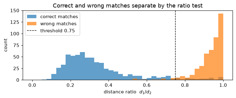Correct matches pile up at low ratios; wrong ones cluster near 1. A threshold around 0.7–0.8 separates them well.

Without filtering, about 41% of nearest neighbors are wrong (mostly keypoints with no true partner in the warped image). A ratio threshold of 0.8 keeps 96% of the correct matches while lifting precision from 59% to 96%. Lowering it to 0.6 gives 99% precision but throws away a tenth of the good matches. Which end you want depends on what comes next: RANSAC tolerates outliers but needs enough inliers, so moderate thresholds (0.7–0.8) are the usual choice.

Brute force versus FLANN on the same descriptors:

bf = cv2.BFMatcher(cv2.NORM_L2)
flann = cv2.FlannBasedMatcher(dict(algorithm=1, trees=5), dict(checks=50))   # 1 = FLANN_INDEX_KDTREE
t0 = time.perf_counter(); m_bf = bf.knnMatch(d1, d2, k=2); t_bf = time.perf_counter() - t0
t0 = time.perf_counter(); m_fl = flann.knnMatch(d1, d2, k=2); t_fl = time.perf_counter() - t0
same = np.mean([a[0].trainIdx == b[0].trainIdx for a, b in zip(m_bf, m_fl)])
print(f"brute force: {t_bf * 1e3:.1f} ms   FLANN: {t_fl * 1e3:.1f} ms   same nearest neighbor: {same:.1%}")

cross = cv2.BFMatcher(cv2.NORM_L2, crossCheck=True).match(d1, d2)
ok = np.linalg.norm(apply_h(H_true, p1[[m.queryIdx for m in cross]]) - p2[[m.trainIdx for m in cross]], axis=1) < 3
print(f"cross-check: {len(cross)} matches, precision {ok.mean():.2f}")

brute force: 2.2 ms   FLANN: 15.8 ms   same nearest neighbor: 91.5%
cross-check: 679 matches, precision 0.92

For a thousand features per image, brute force is both faster and exact. FLANN's tree-building overhead pays off only for large sets (tens of thousands of features, or a database you index once and query many times). Cross-checking helps, but its precision is lower than the ratio test at 0.8. The two filters can also be combined: ratio-test in both directions and keep matches that pass both.

Common mistake: knnMatch returning fewer than two neighbors

knnMatch(d1, d2, k=2) returns a list of lists. If image 2 has only one descriptor, or if a FLANN search comes back short, some inner lists have length 1, and for m, n in knn crashes with "not enough values to unpack". Guard with [p for p in knn if len(p) == 2] in production code. Also, d1 and d2 must both be float32 for FLANN's k-d tree; ORB's uint8 descriptors need the LSH index (algorithm=6).

RANSAC line fitting from scratch

Start with the simplest model: a line through 2D points, with 40% outliers. A line through two points \(\mathbf{p}_1, \mathbf{p}_2\) has unit normal \(\mathbf{n}\) perpendicular to \(\mathbf{p}_2 - \mathbf{p}_1\), and the residual of a point \(\mathbf{p}\) is its perpendicular distance \(|\mathbf{n}^\top(\mathbf{p} - \mathbf{p}_1)|\). The final refit uses total least squares: the best line through a set of points passes through their centroid, with a normal equal to the direction of least variance, the last right singular vector of the centered points.

rng = np.random.default_rng(0)
n_in, n_out = 120, 80
x_in = rng.uniform(0, 10, n_in)
inliers_true = np.column_stack([x_in, 0.5 * x_in + 2 + rng.normal(0, 0.15, n_in)])   # y = 0.5x + 2
outliers_true = rng.uniform([0, 5], [6, 10], size=(n_out, 2))       # clutter in the upper left
pts = np.vstack([inliers_true, outliers_true])
is_inlier_true = np.r_[np.ones(n_in, bool), np.zeros(n_out, bool)]

def fit_line_tls(P):
    """Total least squares line: returns (unit normal n, offset c) with n·p = c."""
    centroid = P.mean(axis=0)
    _, _, Vt = np.linalg.svd(P - centroid)
    n = Vt[-1]
    return n, n @ centroid

def ransac_iterations(w, s, p=0.99):
    return int(np.ceil(np.log(1 - p) / np.log(1 - w ** s)))

def ransac_line(P, t=0.4, p=0.99, w_guess=0.5, rng=None):
    rng = rng or np.random.default_rng(0)
    N = ransac_iterations(w_guess, 2, p)
    best = np.zeros(len(P), bool)
    for _ in range(N):
        i, j = rng.choice(len(P), 2, replace=False)
        d = P[j] - P[i]
        n = np.array([-d[1], d[0]]) / np.linalg.norm(d)     # normal to the line through P[i], P[j]
        inl = np.abs((P - P[i]) @ n) < t
        if inl.sum() > best.sum():
            best = inl
    n, c = fit_line_tls(P[best])                             # refit on all inliers
    return n, c, np.abs(P @ n - c) < t, N

def slope_intercept(n, c):
    return -n[0] / n[1], c / n[1]                            # from n0 x + n1 y = c

n_ls, c_ls = fit_line_tls(pts)
n_r, c_r, inl, N = ransac_line(pts, rng=np.random.default_rng(1))
print(f"iterations used: {N}  (w = 0.5, s = 2, p = 0.99)")
print("least squares on all points: slope %.3f, intercept %.3f" % slope_intercept(n_ls, c_ls))
print("RANSAC + refit:              slope %.3f, intercept %.3f" % slope_intercept(n_r, c_r))
print(f"inliers found: {inl.sum()}, of which truly inliers: {(inl & is_inlier_true).sum()} / {n_in}")

xs = np.linspace(0, 10, 2)
plt.figure(figsize=(6, 3.6))
plt.scatter(*pts[~inl].T, s=10, c="gray", label="RANSAC outliers")
plt.scatter(*pts[inl].T, s=10, c="tab:blue", label="RANSAC inliers")
for (n, c), lab, col in [((n_ls, c_ls), "least squares", "tab:red"), ((n_r, c_r), "RANSAC", "tab:green")]:
    m, b = slope_intercept(n, c)
    plt.plot(xs, m * xs + b, c=col, lw=2, label=lab)
plt.plot(xs, 0.5 * xs + 2, "k:", label="true line")
plt.legend(fontsize=8); plt.title("Line fitting with 40% outliers")
plt.tight_layout(); plt.show()

iterations used: 17  (w = 0.5, s = 2, p = 0.99)
least squares on all points: slope 0.261, intercept 4.749
RANSAC + refit:              slope 0.499, intercept 1.991
inliers found: 119, of which truly inliers: 119 / 120

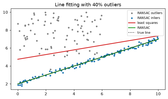Least squares is dragged by the outliers; RANSAC finds the line the inliers agree on, and the refit recovers the true slope and intercept.

Least squares is pulled toward the clutter, with half the true slope. RANSAC found 119 of the 120 true inliers (the one it missed has noise just beyond the 0.4 threshold) and no outliers. An outlier that happened to land within the threshold would have been accepted, and no method could tell it apart from an inlier. Seventeen random pairs were enough, exactly what the formula said for an inlier ratio of 50% (the true ratio here is 60%, so the guess was pessimistic, which is the safe direction).

Checking the iteration formula by simulation

The derivation assumed independent draws. Check it: run many RANSAC "trials" of \(N\) samples each, and measure how often at least one sample is all-inlier.

def p_success_empirical(N, s, n_in, n_total, trials=20000, rng=None):
    rng = rng or np.random.default_rng(0)
    hits = 0
    for _ in range(trials):
        samples = np.array([rng.choice(n_total, s, replace=False) for _ in range(N)])
        hits += np.any(np.all(samples < n_in, axis=1))           # indices < n_in are inliers
    return hits / trials

for s, w_in in [(2, 0.6), (4, 0.6)]:
    N = ransac_iterations(w_in, s, 0.99)
    emp = p_success_empirical(N, s, int(w_in * 200), 200, trials=4000)
    print(f"s={s}, w={w_in}: N={N:3d}  predicted P(success) >= 0.99, simulated {emp:.4f},"
          f" exact formula {1 - (1 - w_in ** s) ** N:.4f}")

s=2, w=0.6: N= 11  predicted P(success) >= 0.99, simulated 0.9928, exact formula 0.9926
s=4, w=0.6: N= 34  predicted P(success) >= 0.99, simulated 0.9895, exact formula 0.9911

The simulation agrees with \(1 - (1 - w^s)^N\) to within sampling noise. (Sampling without replacement within a sample makes all-inlier samples very slightly rarer, which is why the second case lands just under 0.99.)

The DLT from scratch, with Hartley normalization

Now homographies. The implementation follows the derivation exactly: normalize both point sets, build the \(2n \times 9\) matrix, take the last right singular vector, and denormalize.

def normalize_points(P):
    """Similarity T so that T·p has centroid 0 and mean distance sqrt(2). Returns (T, normalized P)."""
    c = P.mean(axis=0)
    scale = np.sqrt(2) / np.mean(np.linalg.norm(P - c, axis=1))
    T = np.array([[scale, 0, -scale * c[0]], [0, scale, -scale * c[1]], [0, 0, 1]])
    return T, apply_h(T, P)

def dlt_homography(src, dst, normalize=True):
    """Homography H with dst ~ H src, from n >= 4 correspondences (Nx2 arrays)."""
    if normalize:
        T1, src = normalize_points(src)
        T2, dst = normalize_points(dst)
    rows = []
    for (x, y), (u, v) in zip(src, dst):
        rows.append([x, y, 1, 0, 0, 0, -u * x, -u * y, -u])
        rows.append([0, 0, 0, x, y, 1, -v * x, -v * y, -v])
    _, _, Vt = np.linalg.svd(np.asarray(rows))
    H = Vt[-1].reshape(3, 3)
    if normalize:
        H = np.linalg.inv(T2) @ H @ T1
    return H / H[2, 2]

# 1) Exact recovery from four noise-free points
H4 = dlt_homography(src, dst)
print("max |H_dlt - H_true| from 4 exact points:", f"{np.abs(H4 - H_true / H_true[2, 2]).max():.2e}")

# 2) Many noisy points: normalized vs unnormalized vs OpenCV (least squares, no RANSAC)
rng = np.random.default_rng(0)
A_pts = rng.uniform([0, 0], [w, h], size=(50, 2))
B_pts = apply_h(H_true, A_pts) + rng.normal(0, 1.0, size=(50, 2))       # 1-pixel noise
grid = np.stack(np.meshgrid(np.linspace(0, w, 10), np.linspace(0, h, 10)), -1).reshape(-1, 2)

def grid_error(H):
    """Mean distance between H and H_true applied to a 10x10 grid over the image (pixels)."""
    return np.linalg.norm(apply_h(H, grid) - apply_h(H_true, grid), axis=1).mean()

H_norm = dlt_homography(A_pts, B_pts, normalize=True)
H_raw = dlt_homography(A_pts, B_pts, normalize=False)
H_cv, _ = cv2.findHomography(A_pts, B_pts, 0)                          # method 0 = all points, least squares
for name, H in [("DLT normalized", H_norm), ("DLT unnormalized", H_raw), ("cv2.findHomography", H_cv)]:
    print(f"{name:20s} mean error vs truth: {grid_error(H):.3f} px")
print(f"max |H_ours - H_cv| (normalized by H[2,2]): {np.abs(H_norm - H_cv / H_cv[2, 2]).max():.2e}")

max |H_dlt - H_true| from 4 exact points: 1.14e-13
DLT normalized       mean error vs truth: 0.355 px
DLT unnormalized     mean error vs truth: 0.405 px
cv2.findHomography   mean error vs truth: 0.346 px
max |H_ours - H_cv| (normalized by H[2,2]): 5.90e-02

Four exact points recover \(\mathbf{H}\) to machine precision. With 1-pixel noise, the normalized DLT and OpenCV land within a hundredth of a pixel of each other in accuracy (the largest entry difference, 0.06, is in the translation entries, which are about 40). The unnormalized version is about 15% worse here, and the gap grows with image size and noise (try it with coordinates at 4K resolution).

RANSAC for homographies, from scratch

Now combine the two: RANSAC with the 4-point DLT as the minimal solver, reprojection error as the residual, adaptive iteration count, and a final normalized-DLT refit on all inliers. Run it on the ratio-tested SIFT matches from the warped astronaut, and compare with OpenCV's RANSAC and MAGSAC.

def ransac_homography(src, dst, thresh=3.0, p=0.999, max_iters=5000, rng=None):
    """Adaptive RANSAC with the 4-point DLT. Returns (H, inlier mask, iterations run)."""
    rng = rng or np.random.default_rng(0)
    n = len(src)
    best_inl, N, i = np.zeros(n, bool), max_iters, 0
    while i < min(N, max_iters):
        idx = rng.choice(n, 4, replace=False)
        H = dlt_homography(src[idx], dst[idx])
        if not np.all(np.isfinite(H)):
            i += 1; continue
        err = np.linalg.norm(apply_h(H, src) - dst, axis=1)
        inl = err < thresh
        if inl.sum() > best_inl.sum():
            best_inl = inl
            w_hat = inl.mean()                                 # update the inlier-ratio estimate
            N = ransac_iterations(min(w_hat, 0.999999), 4, p) if w_hat > 0 else max_iters
        i += 1
    H = dlt_homography(src[best_inl], dst[best_inl])          # refit on all inliers
    inl = np.linalg.norm(apply_h(H, src) - dst, axis=1) < thresh
    return H, inl, i

good = [m for m, n in knn if m.distance < 0.8 * n.distance]
s_pts = p1[[m.queryIdx for m in good]]; d_pts = p2[[m.trainIdx for m in good]]
H_r, inl_r, iters = ransac_homography(s_pts, d_pts, rng=np.random.default_rng(0))
H_cv, mask_cv = cv2.findHomography(s_pts, d_pts, cv2.RANSAC, 3.0)
H_mag, mask_mag = cv2.findHomography(s_pts, d_pts, cv2.USAC_MAGSAC, 3.0)
H_ls, _ = cv2.findHomography(s_pts, d_pts, 0)
print(f"{len(good)} matches after ratio test; our RANSAC ran {iters} iterations")
for name, H, ninl in [("least squares (no RANSAC)", H_ls, None), ("ours", H_r, inl_r.sum()),
                      ("cv2.RANSAC", H_cv, mask_cv.sum()), ("cv2.USAC_MAGSAC", H_mag, mask_mag.sum())]:
    extra = f"{ninl:4d} inliers" if ninl is not None else "    all points"
    print(f"{name:26s} {extra}   error vs truth {grid_error(H):7.3f} px")

651 matches after ratio test; our RANSAC ran 4 iterations
least squares (no RANSAC)      all points   error vs truth   2.026 px
ours                        623 inliers   error vs truth   0.078 px
cv2.RANSAC                  623 inliers   error vs truth   0.077 px
cv2.USAC_MAGSAC             623 inliers   error vs truth   0.110 px

With about 4% outliers, least squares is off by 2 pixels on average, while all three robust estimators land within about a tenth of a pixel; the differences among them are at the level of noise. The adaptive loop stopped after 4 iterations because the first clean sample revealed an inlier ratio near 96%, for which the formula asks for only a handful of samples. OpenCV additionally refines the final \(\mathbf{H}\) by minimizing reprojection error (Levenberg-Marquardt) rather than the DLT's algebraic error, which matters more when matches are fewer or noisier.

Common mistake: swapping source and destination

cv2.findHomography(srcPoints, dstPoints) returns \(\mathbf{H}\) with \(\text{dst} \sim \mathbf{H}\,\text{src}\). In a match, queryIdx indexes the descriptors you passed first to the matcher and trainIdx the second. If you build src from trainIdx by accident, you get \(\mathbf{H}^{-1}\), and warpPerspective warps your image in the wrong direction. When a warp looks "inverted", check this first.

A panorama from overlapping crops

To stitch with known ground truth, cut two overlapping views from the wide rocket image. The left view is columns 0–419. The right view is columns 220–639, warped by a perspective transform (as if the camera had turned slightly) and made 15% brighter (as if auto-exposure had changed). Because you built the right view yourself, you know the true homography that maps it back into the left view's frame.

from skimage import data

scene = data.rocket()                                   # RGB, 427 x 640
H_s, W_s = scene.shape[:2]
x0 = 220
left = scene[:, :420].copy()
right_raw = scene[:, x0:].copy()
hr, wr = right_raw.shape[:2]
P = cv2.getPerspectiveTransform(np.float32([[0, 0], [wr, 0], [wr, hr], [0, hr]]),
                                np.float32([[0, 25], [wr - 10, 0], [wr, hr], [12, hr - 30]]))
right = cv2.warpPerspective(right_raw, P, (wr, hr))
right_valid = cv2.warpPerspective(np.full((hr, wr), 255, np.uint8), P, (wr, hr))   # where the view has content
right = np.clip(right.astype(np.float32) * 1.15 + 5, 0, 255).astype(np.uint8)

# Ground truth: a right-view pixel maps back through P^-1, then shifts by x0 into the left frame.
T_x0 = np.array([[1, 0, x0], [0, 1, 0], [0, 0, 1.0]])
H_gt = T_x0 @ np.linalg.inv(P)
H_gt /= H_gt[2, 2]

g_l, g_r = (cv2.cvtColor(im, cv2.COLOR_RGB2GRAY) for im in (left, right))
kl, dl = sift.detectAndCompute(g_l, None)
kr, dr = sift.detectAndCompute(g_r, None)
good = [m for m, n in cv2.BFMatcher(cv2.NORM_L2).knnMatch(dr, dl, k=2) if m.distance < 0.75 * n.distance]
src_r = np.float32([kr[m.queryIdx].pt for m in good])       # points in the right view
dst_l = np.float32([kl[m.trainIdx].pt for m in good])       # their matches in the left view
H_est, inl, iters = ransac_homography(src_r, dst_l, thresh=2.0, rng=np.random.default_rng(0))

view_grid = np.stack(np.meshgrid(np.linspace(0, wr, 30), np.linspace(0, hr, 30)), -1).reshape(-1, 2)
reproj = np.linalg.norm(apply_h(H_est, view_grid) - apply_h(H_gt, view_grid), axis=1)
in_overlap = apply_h(H_gt, view_grid)[:, 0] < 420           # grid points that land inside the left view
print(f"keypoints left/right: {len(kl)}/{len(kr)}, ratio-test matches: {len(good)}, inliers: {inl.sum()}")
print(f"error vs true H in the overlap:   mean {reproj[in_overlap].mean():.2f} px, max {reproj[in_overlap].max():.2f} px")
print(f"error vs true H beyond the overlap: mean {reproj[~in_overlap].mean():.2f} px, max {reproj[~in_overlap].max():.2f} px")

vis = cv2.drawMatches(left, kl, right, kr, [cv2.DMatch(m.trainIdx, m.queryIdx, 0) for m, ok in zip(good, inl) if ok],
                      None, matchColor=(0, 255, 0), flags=cv2.DRAW_MATCHES_FLAGS_NOT_DRAW_SINGLE_POINTS)
plt.figure(figsize=(10, 3.6)); plt.imshow(vis); plt.axis("off")
plt.title("Left view and perspective-warped, brighter right view: RANSAC inlier matches")
plt.tight_layout(); plt.show()

keypoints left/right: 281/235, ratio-test matches: 55, inliers: 50
error vs true H in the overlap:   mean 0.40 px, max 1.55 px
error vs true H beyond the overlap: mean 2.51 px, max 5.18 px

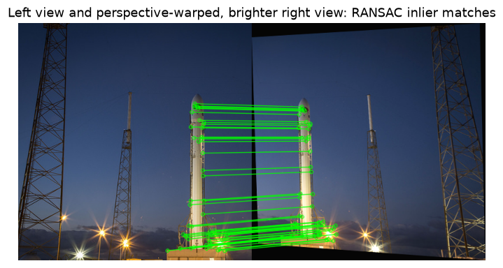Inlier matches all fall in the shared 200-column overlap, despite the perspective and exposure change.

Inside the overlap, where the matches are, the estimated homography is within half a pixel of the truth on average. Beyond the overlap it extrapolates, and the error grows to a few pixels at the far edge of the right view. That's a general property of fitted transforms: they're accurate where the data is. Spreading matches over the whole image (or chaining through more overlapping views) keeps the extrapolation short. Now build the canvas, warp both views onto it, and compare a naive paste with feathered blending.

def warp_to_canvas(images, homographies, valid=None):
    """Warp each image (and its validity mask) into a shared canvas. Returns warped images and masks."""
    corners = []
    for im, H in zip(images, homographies):
        hh, ww = im.shape[:2]
        corners.append(apply_h(H, np.float32([[0, 0], [ww, 0], [ww, hh], [0, hh]])))
    corners = np.vstack(corners)
    xmin, ymin = np.floor(corners.min(axis=0)).astype(int)
    xmax, ymax = np.ceil(corners.max(axis=0)).astype(int)
    T = np.array([[1, 0, -xmin], [0, 1, -ymin], [0, 0, 1.0]])          # shift so the canvas starts at 0
    size = (xmax - xmin, ymax - ymin)
    warped, masks = [], []
    valid = valid or [np.full(im.shape[:2], 255, np.uint8) for im in images]
    for im, H, v in zip(images, homographies, valid):
        warped.append(cv2.warpPerspective(im, T @ H, size).astype(np.float32))
        masks.append(cv2.warpPerspective(v, T @ H, size, flags=cv2.INTER_NEAREST))
    return warped, masks, T

def feather_blend(warped, masks):
    weights = [cv2.distanceTransform((m > 0).astype(np.uint8), cv2.DIST_L2, 5) for m in masks]
    num = sum(wt[..., None] * im for wt, im in zip(weights, warped))
    den = sum(weights)[..., None]
    return np.clip(num / np.maximum(den, 1e-6), 0, 255).astype(np.uint8)

warped, masks, T_canvas = warp_to_canvas([left, right], [np.eye(3), H_est],
                                         valid=[np.full(left.shape[:2], 255, np.uint8), right_valid])
naive = warped[0].copy()
naive[masks[1] > 0] = warped[1][masks[1] > 0]                           # paste right over left
naive = np.clip(naive, 0, 255).astype(np.uint8)
blended = feather_blend(warped, masks)

st = cv2.Stitcher_create(cv2.Stitcher_PANORAMA)
status, pano_cv = st.stitch([cv2.cvtColor(left, cv2.COLOR_RGB2BGR), cv2.cvtColor(right, cv2.COLOR_RGB2BGR)])
print("canvas size (h, w):", naive.shape[:2], " canvas offset:", T_canvas[:2, 2],
      "  cv2.Stitcher status:", status,
      "(0 = OK)  output (h, w):", pano_cv.shape[:2])

fig, axes = plt.subplots(1, 3, figsize=(10, 3.3))
axes[0].imshow(naive); axes[0].set_title("Naive paste", fontsize=10)
axes[1].imshow(blended); axes[1].set_title("Feathered blend (our H)", fontsize=10)
axes[2].imshow(cv2.cvtColor(pano_cv, cv2.COLOR_BGR2RGB)); axes[2].set_title("cv2.Stitcher", fontsize=10)
for ax in axes: ax.axis("off")
plt.tight_layout(); plt.show()

canvas size (h, w): (494, 645)  canvas offset: [ 0. 30.]   cv2.Stitcher status: 0 (0 = OK)  output (h, w): (452, 750)

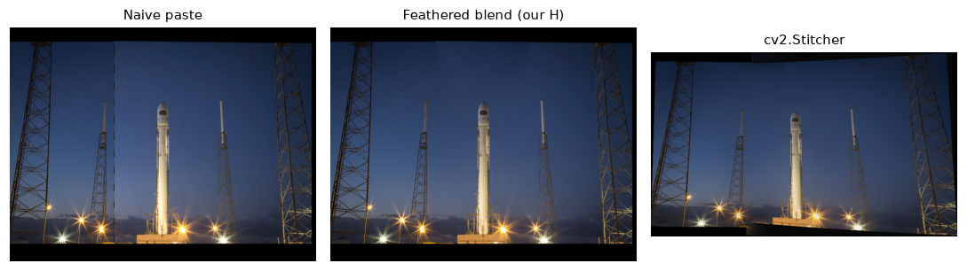The naive paste shows a hard brightness step at the right view's border; feathering hides it by fading between the two views; OpenCV's Stitcher also blends well but reprojects onto a sphere, so its output is curved and larger.

The canvas is slightly larger than the original \(427 \times 640\) scene and starts 30 pixels above it, because the right view's full rectangle (including the black corners that the simulated perspective change introduced) maps to a quadrilateral that sticks out above and below the original. The validity masks keep those black regions out of the blend. cv2.Stitcher gets there without being told anything, but its result isn't directly comparable pixel by pixel: in PANORAMA mode it estimates a focal length and camera rotations, warps onto a sphere, compensates exposure, finds seams, and uses multi-band blending.

Common mistake: forgetting the canvas translation

If you warp the right view with warpPerspective(right, H, (W, H)) directly, any part that maps to negative coordinates is silently cut off, because the output image starts at \((0, 0)\). Always compute where the corners go, then prepend the translation T to every homography, as in warp_to_canvas.

Exercises

Exercise 1: RANSAC iterations by hand (easy)

Using \(N = \lceil \log(1 - p) / \log(1 - w^s) \rceil\):

1. How many iterations does a homography (\(s = 4\)) need with 50% inliers at \(p = 0.99\)?
2. How does that change at \(p = 0.999\)?
3. A colleague proposes estimating the homography from 6 points per sample "for robustness". How many iterations does that need at 50% inliers and \(p = 0.99\)?

Solution

1. \(w^s = 0.5^4 = 0.0625\). \(N = \log(0.01) / \log(0.9375) = -4.605 / -0.0645 = 71.4\), so 72.
2. \(N = \log(0.001) / \log(0.9375) = -6.908 / -0.0645 = 107.0\), so 108: the extra "9" of confidence costs only 50% more iterations, because \(N\) grows with \(\log(1/(1-p))\).
3. \(w^s = 0.5^6 = 0.0156\). \(N = -4.605 / \log(0.984375) = -4.605 / -0.01575 = 292.4\), so 293, four times more. Larger samples are more likely to be contaminated. Robustness to noise comes from the final refit on all inliers, not from bigger samples.

for p, s in [(0.99, 4), (0.999, 4), (0.99, 6)]:
    print(p, s, ransac_iterations(0.5, s, p))

0.99 4 72
0.999 4 108
0.99 6 293

Exercise 2: Why ratio and not distance? (easy)

A shelf image contains 40 identical cereal boxes. Explain what the ratio test does to matches on the boxes, and why that's usually what you want for estimating a homography. When would it be a problem?

Solution

Each keypoint on one box has near-identical descriptors on the other 39 boxes, so its nearest and second-nearest distances are almost equal and the ratio is close to 1. The ratio test rejects nearly all of these matches. That's desirable for geometry: a match from box 3 to box 7 is an outlier, and keeping dozens of such ambiguous matches would lower the inlier ratio and could even produce a coherent wrong model (all boxes shifted by one position). It's a problem when the repeated structure is all there is: a building facade of identical windows or a tiled floor may leave too few matches. Then you can relax the ratio, keep the top-\(k\) candidates per keypoint and let RANSAC choose, or use guided matching (estimate a rough model from the few distinctive matches, then search near the predicted positions).

Exercise 3: The DLT needs four points in general position (medium)

Build the \(8 \times 9\) DLT matrix \(\mathbf{A}\) (without normalization) for (a) four points at the corners of a \(100 \times 100\) square and (b) four points of which three are collinear. In both cases, use the targets \(\mathbf{H}_{\text{true}}\mathbf{x}\) so that an exact homography exists. Compute the singular values of \(\mathbf{A}\). What do you see, and what does it mean for the solution?

Solution

With four points in general position, \(\mathbf{A}\) has rank 8, so its null space is one-dimensional: a unique \(\mathbf{H}\) up to scale. With three collinear points, the equations from those three points are partly redundant (a homography maps lines to lines, so knowing where two of them go already constrains the third), the rank drops to 7, and the null space becomes two-dimensional: infinitely many homographies fit the four correspondences.

def dlt_matrix(src_pts, dst_pts):
    rows = []
    for (x, y), (u, v) in zip(src_pts, dst_pts):
        rows += [[x, y, 1, 0, 0, 0, -u * x, -u * y, -u], [0, 0, 0, x, y, 1, -v * x, -v * y, -v]]
    return np.array(rows, float)

square = np.array([[0, 0], [100, 0], [100, 100], [0, 100]], float)
collinear = np.array([[0, 0], [100, 100], [200, 200], [0, 100]], float)   # first three on y = x
for name, P4 in [("square", square), ("three collinear", collinear)]:
    sv = np.linalg.svd(dlt_matrix(P4, apply_h(H_true, P4)), compute_uv=False)
    print(f"{name:16s} smallest singular values: {sv[-3:]}")

square           smallest singular values: [43.4191258  16.02306942  0.99990262]
three collinear  smallest singular values: [2.52336276e+01 1.09117968e+00 2.72389949e-13]

An \(8 \times 9\) matrix has 8 singular values, and a 9th null direction always exists. For the square, the 8th singular value is clearly nonzero (rank 8), leaving exactly one null vector: the homography. With three collinear points the 8th singular value drops to numerical zero, so the null space is two-dimensional and the homography is not determined. RANSAC implementations check for collinear samples and skip them; the next random sample is almost always fine.

Exercise 4: Gain compensation (medium)

The right view in the panorama was 15% brighter. Estimate a single gain \(g\) for the right view that best matches the left view in the overlap, in the least-squares sense: minimize \(\sum_{\mathbf{x} \in \text{overlap}} (g\,I_r(\mathbf{x}) - I_l(\mathbf{x}))^2\). Derive the closed-form \(g\), apply it before blending, and report the mean absolute difference between the two warped views in the overlap before and after.

Solution

Setting the derivative with respect to \(g\) to zero gives \(g = \sum I_r I_l / \sum I_r^2\).

ov = (masks[0] > 0) & (masks[1] > 0)
Il, Ir = warped[0][ov], warped[1][ov]
g = (Ir * Il).sum() / (Ir * Ir).sum()
print(f"gain {g:.3f}")
print(f"mean |difference| in overlap: before {np.abs(Ir - Il).mean():.2f}, after {np.abs(g * Ir - Il).mean():.2f}")

gain 0.840
mean |difference| in overlap: before 15.97, after 2.89

The gain is close to \(1/1.15 = 0.87\) (the small offset of 5 and the clipping at 255 account for the rest). The remaining difference is interpolation (the right view was resampled twice) plus the offset. Real stitchers estimate one gain per image jointly over all overlaps, with a prior that keeps gains near 1, so the whole panorama doesn't drift darker or brighter.

Exercise 5: Robustness breakdown (hard)

Using ransac_homography, find the outlier fraction at which RANSAC starts to fail on synthetic data. Generate 200 correspondences from H_true with 1-pixel noise, replace a fraction \(f\) of the destinations with uniform random points, and for \(f \in \{0.5, 0.7, 0.8, 0.9, 0.95\}\) run your RANSAC with max_iters=2000 over 20 seeds. Report the median grid error and the fraction of runs with error under 5 pixels. Then explain the result using the iteration formula.

Solution

rng = np.random.default_rng(0)
A0 = rng.uniform([0, 0], [w, h], size=(200, 2))
B0 = apply_h(H_true, A0) + rng.normal(0, 1.0, size=(200, 2))
for f in [0.5, 0.7, 0.8, 0.9, 0.95]:
    errs = []
    for seed in range(20):
        r = np.random.default_rng(seed)
        B = B0.copy()
        bad = r.choice(200, int(f * 200), replace=False)
        B[bad] = r.uniform([0, 0], [w, h], size=(len(bad), 2))
        H_f, _, _ = ransac_homography(A0, B, thresh=3.0, max_iters=2000, rng=r)
        errs.append(grid_error(H_f))
    errs = np.array(errs)
    print(f"outliers {f:.0%}: median error {np.median(errs):8.2f} px, success rate {(errs < 5).mean():.0%},"
          f" needed N = {ransac_iterations(1 - f, 4, 0.999)}")

outliers 50%: median error     0.35 px, success rate 100%, needed N = 108
outliers 70%: median error     0.50 px, success rate 100%, needed N = 850
outliers 80%: median error     1.40 px, success rate 85%, needed N = 4314
outliers 90%: median error   333.30 px, success rate 5%, needed N = 69075
outliers 95%: median error   356.34 px, success rate 0%, needed N = 1105238

RANSAC is reliable up to 70% outliers, mostly works at 80%, and collapses at 90% and beyond. The iteration cap explains it. With max_iters=2000, the probability of drawing at least one clean 4-point sample is \(1 - (1 - w^4)^{2000}\):

• \(w = 0.3\): \(w^4 = 0.0081\), success probability essentially 1.
• \(w = 0.2\): \(w^4 = 0.0016\), success probability \(1 - e^{-3.2} \approx 0.96\). The observed 85% is a little lower because, with only 40 inliers and 1-pixel noise, some clean samples are badly conditioned (points close together) and yield a model that misses part of the inlier set.
• \(w = 0.1\): \(w^4 = 10^{-4}\), success probability \(1 - e^{-0.2} \approx 0.18\), and the observed 5% is lower still for the same reason.
• \(w = 0.05\): \(w^4 \approx 6 \times 10^{-6}\), about 1%. Worse, with only 10 inliers among 200 points, a wrong homography can collect a comparable number of scattered outliers within 3 pixels by chance, so even a clean sample might not win.

The formula's last column shows the fix in principle (tens of thousands of iterations for 90% outliers), and also why nobody does that in practice: improve the matching instead (a stricter ratio test, cross-checking, PROSAC ordering by match quality) so that RANSAC never sees such a low inlier ratio.

Check yourself

1. Why is the ratio test more reliable than a fixed threshold on descriptor distance?

   Answer

   Absolute distances vary with texture, noise, and viewpoint, so no single threshold separates correct from wrong matches everywhere. The ratio compares a match with the best alternative for the same keypoint: correct matches are much closer than any alternative (low ratio), while wrong or ambiguous matches are about as close as the runner-up (ratio near 1).

2. When should you use brute-force matching, and when FLANN or another ANN index?

   Answer

   Brute force for typical image pairs (up to a few thousand features each): it's exact and fast enough. ANN when one side is very large, such as a database of millions of descriptors, or when the same index is queried many times.

3. Derive the RANSAC iteration count \(N\) in one line, and say which quantity it depends on most strongly.

   Answer

   The probability that all \(N\) samples of size \(s\) contain an outlier is \((1 - w^s)^N\); setting it \(\le 1 - p\) gives \(N \ge \log(1-p)/\log(1 - w^s)\). It depends exponentially on the sample size \(s\) through \(w^s\), and very strongly on the inlier ratio \(w\). It doesn't depend on the number of points.

4. Why does least squares fail with outliers, while RANSAC doesn't?

   Answer

   Least squares minimizes the sum of squared residuals, so a single large residual dominates and pulls the fit (breakdown point 0). RANSAC fits minimal samples and scores hypotheses by how many points agree within a threshold; outliers only add a bounded penalty (they're simply not counted), so as long as some sample is clean, the right model wins.

5. How many correspondences does a homography need, and why must the DLT points be normalized?

   Answer

   Four, in general position (no three collinear): 8 degrees of freedom, 2 equations per point. Normalization (centroid at the origin, mean distance \(\sqrt{2}\)) makes the entries of the DLT matrix comparable in magnitude; with raw pixel coordinates the matrix is badly conditioned, and the solution is unnecessarily sensitive to noise.

6. Why are images from a camera rotating about its center related by a homography regardless of the scene's 3D structure?

   Answer

   With no translation, a scene point's depth doesn't affect where it appears: each pixel corresponds to a ray, and rotating the camera just maps rays to rays through the same center. That ray-to-ray mapping is \(\mathbf{K}'\mathbf{R}\mathbf{K}^{-1}\), a \(3 \times 3\) homography (derived in the next chapter). Any translation introduces parallax, which no homography can model unless the scene is planar.

7. What does feathering do, and what artifact does multi-band blending avoid that feathering can produce?

   Answer

   Feathering weights each image by its distance to its own border, so contributions fade smoothly across the overlap and exposure seams disappear. With a wide transition, though, slightly misaligned fine details (or moving objects) appear doubled (ghosting). Multi-band blending uses narrow transitions for high frequencies and wide ones for low frequencies, avoiding both seams and ghosting.

Key takeaways

• Use L2 distance for SIFT-like float descriptors and Hamming distance for binary ones. Brute force is exact and fast for image pairs; ANN indexes (FLANN, LSH, HNSW) pay off for large databases.
• The ratio test (keep matches with \(d_1/d_2 < 0.7\)–\(0.8\)) removes most wrong and ambiguous matches at a small cost in recall.
• Least squares breaks down with a single gross outlier. RANSAC fits minimal samples and keeps the hypothesis with the largest consensus set, then refits on its inliers.
• RANSAC needs \(N = \lceil\log(1-p)/\log(1-w^s)\rceil\) iterations: independent of the number of points, exponential in the sample size, and very sensitive to the inlier ratio.
• The DLT turns \(\mathbf{x}' \sim \mathbf{H}\mathbf{x}\) into a linear system \(\mathbf{A}\mathbf{h} = \mathbf{0}\) solved by SVD. Normalize the points first, and refine on reprojection error if accuracy matters.
• A panorama is: match, RANSAC homography, warp onto a translated canvas (or a cylinder or sphere for wide pans), compensate exposure, and blend.

Further reading

• M. A. Fischler and R. C. Bolles, "Random Sample Consensus: A Paradigm for Model Fitting with Applications to Image Analysis and Automated Cartography," Communications of the ACM, 24(6), 1981.
• R. Hartley and A. Zisserman, Multiple View Geometry in Computer Vision, 2nd ed., Cambridge University Press, 2004, chapter 4 (homography estimation, the DLT, normalization, and RANSAC).
• M. Brown and D. G. Lowe, "Automatic Panoramic Image Stitching using Invariant Features," International Journal of Computer Vision, 74(1), 2007. The design behind OpenCV's Stitcher.
• P. J. Burt and E. H. Adelson, "A Multiresolution Spline with Application to Image Mosaics," ACM Transactions on Graphics, 2(4), 1983.
• OpenCV documentation, "Feature Matching" and "Feature Matching + Homography to find Objects" tutorials, at docs.opencv.org.

Next

Homographies describe planes and rotating cameras. To go further, to measure real distances, place virtual objects, and reason about 3D, you need a model of the camera itself. Continue with Cameras and calibration.